20+ Excel Table tricks to turbo charge your data

20+ Excel Table tricks to turbo charge your data
Following are the tricks you can do with the features Excel tables offer. Following list is in no particular order. I think all of them are handy that every excel user must know to make his/her work more easy.
Excel Trick # 1. You name it!
Each table bears a unique name. And once something has a name it not only has identity it has authority as well. Same is the case with tables. Once given the name you can step into the realm of structured referencing instead of orthodox column row reference system. With the names being automatically generated it is easier for you to navigate to that data. For instance you have sales results of 10 different products then jumping from one to other will be so cumbersome. But with names defined you can jump to it easily by selecting the table from name box. Following animation illustrates the same where one workbook has several tables on several worksheets and you can jump to each table easily
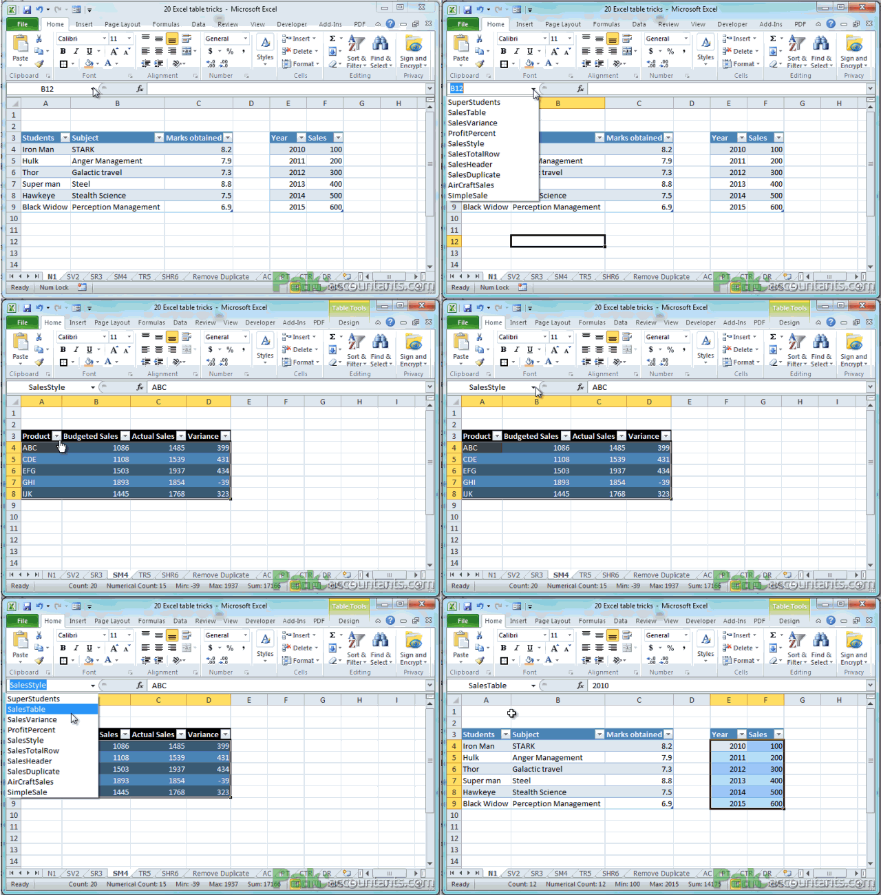
Another feature that comes with it is that normally a named range is fixed and stays to the extent you mention while naming it. However, with tables it can grow as data grows and it shrinks as data volume regresses. So you don’t have to use OFFSET functions and all that mess in many instances. This will be further discussed in Structured references and dynamic ranges in upcoming tricks.
Excel Table Trick # 2. Resize as you advise! Without affecting other areas of worksheet
Already have the table and want to increase or decrease the number of rows and columns from it without affecting the other parts of worksheet. Consider it done!
You can do this by either of the following ways:
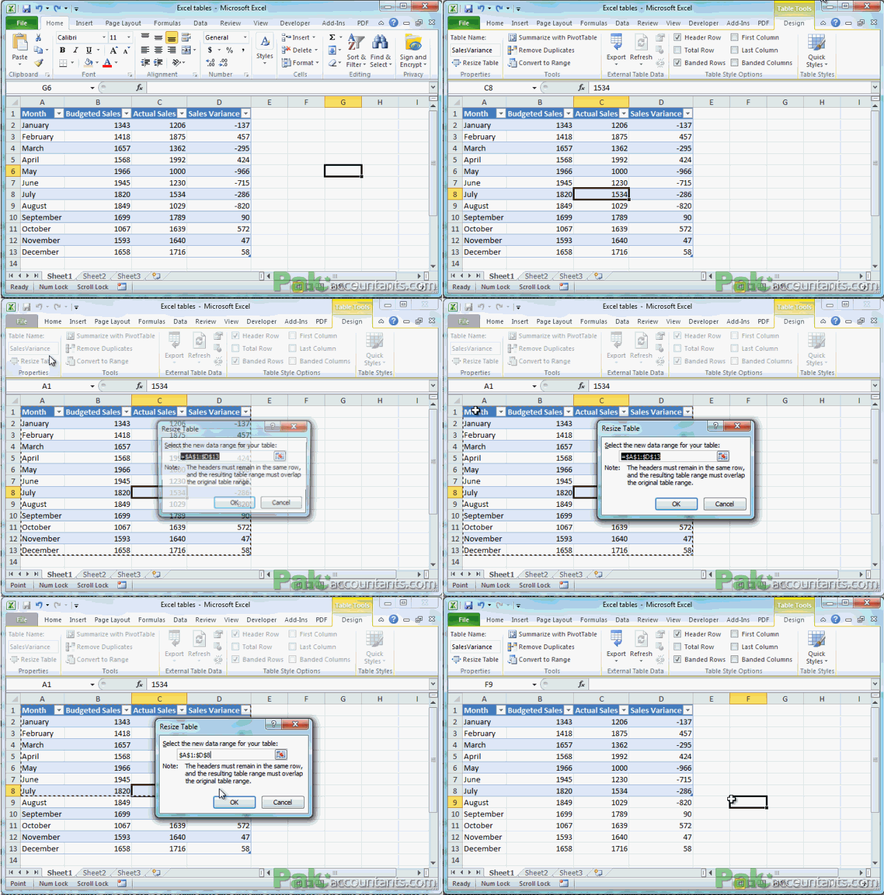
Have an active cell with in the table and go to contextual tab. In the Properties group click resize table button and make a fresh selection to include or exclude certain rows and/or columns. Remember you have to make the selection from the first cell of the table otherwise Excel will give an error. Remember even if you exclude certain part of table from new selection, data won’t get deleted its just that its not part of the table anymore. If you don’t want to keep it you will have to delete that manually.
Use the resize handler at the bottom right corner of the table. Click and drag and it will extend or exclude rows/columns for you from the table. Remember if you add new columns and they don’t have the headers already written then Excel will put in the generic headers as Column1, Column2 and so on. If you exclude certain rows and columns data won’t be deleted and you have to do it manually if you want to.
Use right click menu to insert or delete rows and columns. It works the same way as it is in case of normal rows and columns of worksheet but inside table it will affect table only and leave the other items in worksheet in their place.
Excel Table Trick # 3. Structured references
My personal favourite feature of tables and beyond doubt it is one big advancement. For example you want to calculate the average per unit profit on the sales made so far.
To do it as per normal way follow these steps:
Step 1: Open tab named SR3 and in cell E4 put the following formula to calculate total revenue generated:
=C4*D4
Step 2: Drag the fill handler to paste the apply similar formula to next cells. Remember as cell reference is relative so it will auto update as you drag it to next rows. Doing it successfully will give you total revenue.
Step 3: In cell G4 put this formula to calculate profit margin:
=(E4-F4)/E4*100
Step 4: Executing the third step will give you profit margin in decimals. To round it up to 0 decimal place replace the formula in G4 with this:
=ROUND((E4-F4)/E4*100,0)
We have simply enclosed the whole calculation inside round function to round the figure to integer i.e. zero decimal place. Drag the fill handler to populate rest of the cells or simply double click it.
To do it using structured references follow these steps:
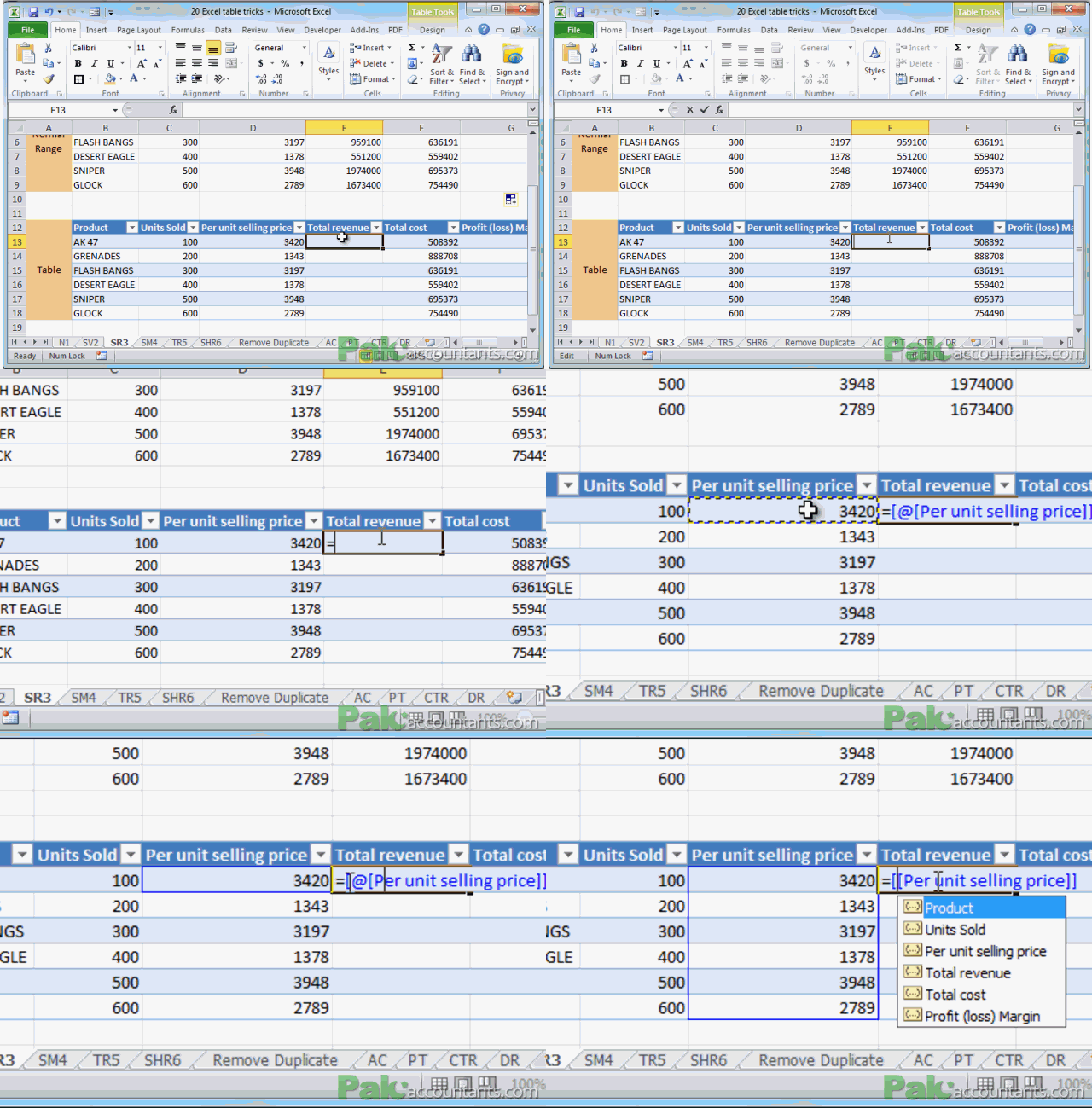
Step 1: having SR3 tab still active scroll down to cell E13 press F2 to enter edit mode and hit “=” key on the keyboard. Click on cell D13 and you will notice that formula will look like this: =[@[Per unit selling price]]
Instead of having =D13 why are we getting it? well this is called structured reference system which is part of table feature in Excel. It uses table name and column names to identify the data for function to operate instead of cell references. [Per unit selling price] is an address in itself. Remember to represent table columns excel uses square brackets [ ]. @ sign means “at this row” that means it will not consider the whole per unit selling price column. If we remove @ sign you will observe that active area expands to whole column. Consider following animation to understand this phenomena:
Back to our calculation.
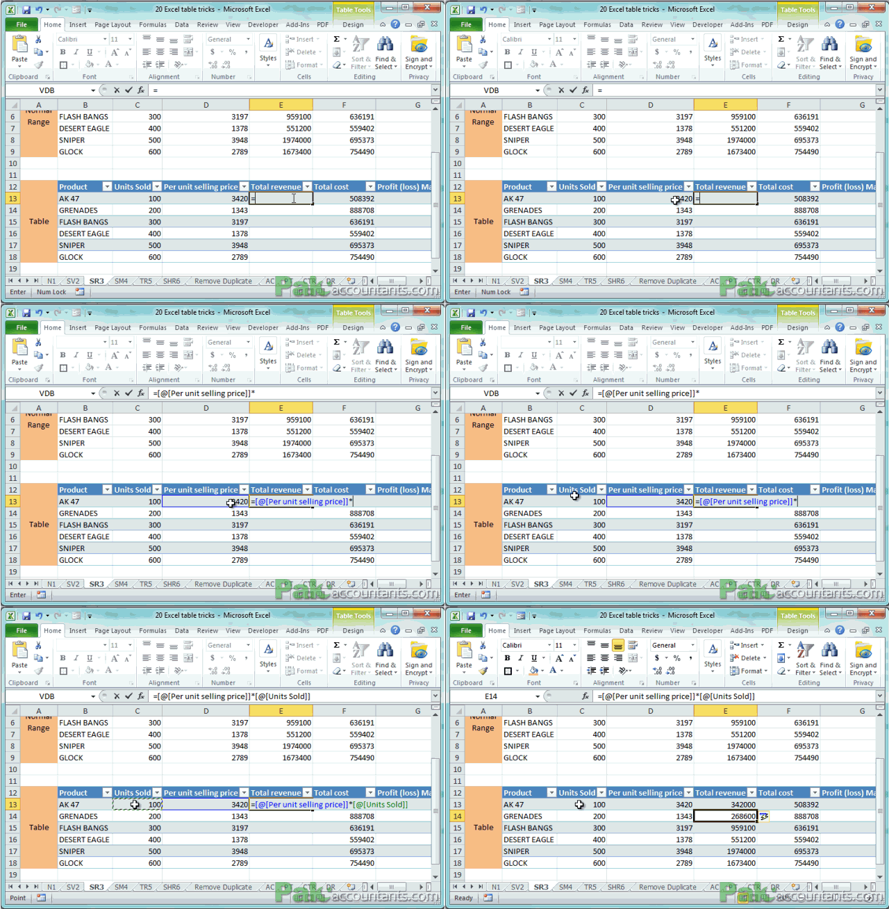
Step 2: Make sure you have done step 1 until you get: =[@[Per unit selling price]]. Hit “*” asterisk key on the keyboard and click cell C13. Press Enter. It will give you total sales revenue figure. The moment you hit Enter the whole column will be done for you automatically. This is called calculated column feature of Excel. It will be explained further below. Watch the following video to correctly execute this step:
Step 3: Go to cell G13. Press F2 to enter edit mode. Press equals button on the keyboard. Start writing ROUND, just when you will be typing a helper list will appear and instead of writing ROUND completely use directional keys to select the function from the list and hit TAB key to insert the function in the cell. Do not press Enter to insert function as Enter key completes input.
Step 2: Once you have =ROUND( in cell G13 and still in edit mode, punch in Shift+9 to put “(” open bracket.
Step 3: Click cell E13 press minus or dash button on keyboard and click F13. Hit Shift+0 to put close bracket.
Step 4: Press “/” key on the keyboard to put hash or divide by sign and click cell E13 again.
Step 5: Put asterisk and punch in 100. Hit comma to jump to second ROUND formula’s requirement field and type 0 i.e. zero. Press Shift+0 again to close the formula and hit Enter key.
Consider following animation to execute these steps properly
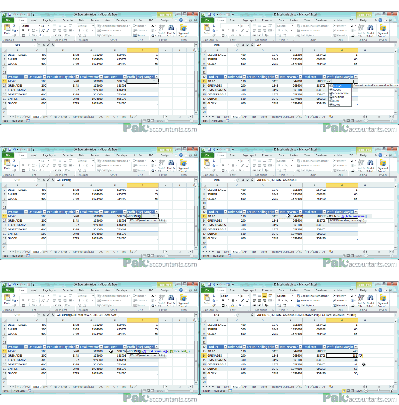
You will get the same profit percentage results as you get in normal range. But look at the formula. That is completely different makes much more sense. As you can understand what is being multiplied and what is being divided by whom. This goes hand in hand with your theoretical knowledge of calculating profit margin as well.
A detailed article on structured references and how to use it will be available soon 🙂
Excel Table Trick # 4. Calculated columns
Insert a formula in a single cell within a column and table will automatically insert that formula for you in the rest of the column instantly saving you the hassle of dragging and copy/paste. This not only reduce inefficiencies and errors but also help keeping the consistency within in data. You have seen it in action in trick 3 when you press enter and the whole column gets the profit margin calculated automatically.
Don’t want calculated columns to be done automatically? Use smart tag to revert it or turn it off altogether from excel’s options.
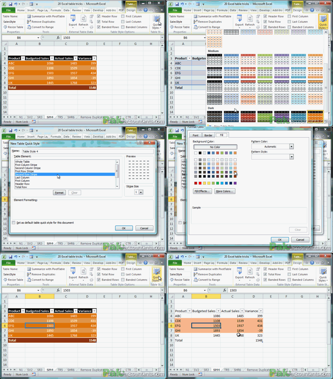
Excel Table Trick # 5. Endless table styles
Everyone likes good numbers. But good numbers in good style is an extra topping not to miss. From quick style library you can select some built in styles quickly or make your own even to suit your needs.
Excel Table Trick # 6. Get filter and sort by default
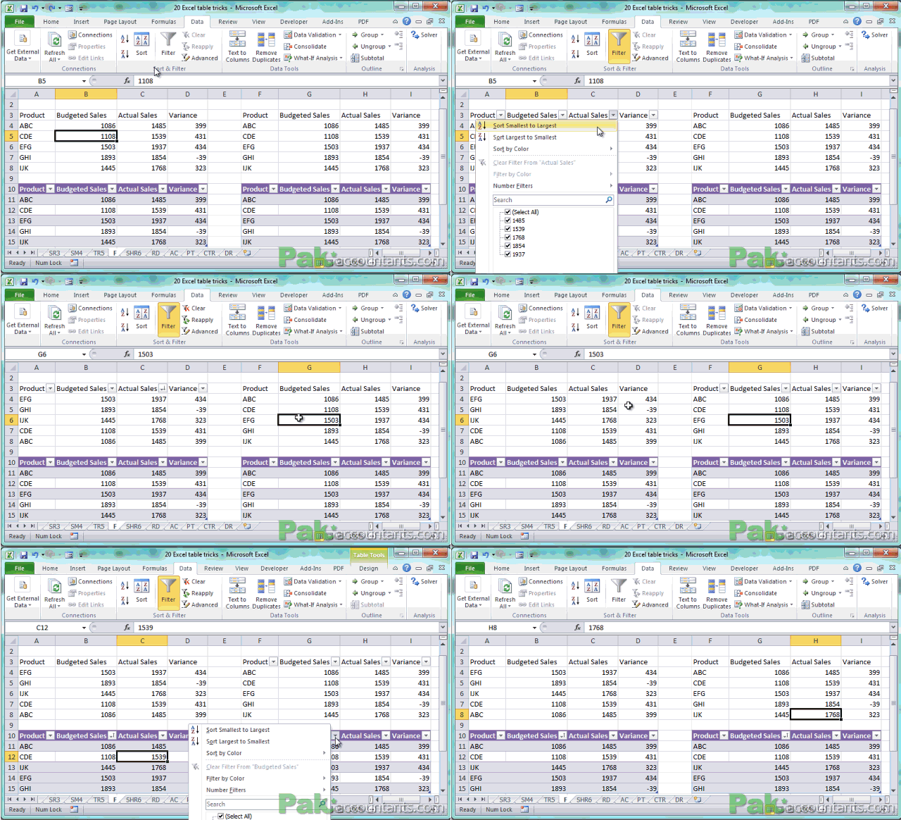
Every table gets the filter and sort option turned on by default and let you filter the result on the fly easily. And one fascinating thing is that each table gets its own sort and filter option and filters can be applied on multiple tables even if they are on the same worksheet. Normally only one data range can be filtered at a time in the worksheet.
Excel Table Trick # 7. Dedicated row loaded with formula
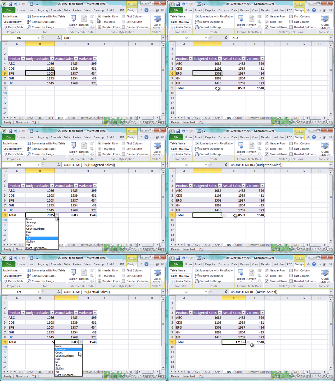
On click of a button you get a dedicated row that comes loaded with formula. And a little formatting is done for you as well so that it stands out from the rest of the data.
Although it is called total row and by default sums up the values to give the total but one does have several options to select from the drop down menu and it definitely not limited to given formula you can insert your own formula.
Excel Table Trick # 8. Remove duplicate options by default
Although this does not count as a separate trick but still mentioning it as it appears in table contextual tab. I tried to find some unique use of this with tables that is different from normal remove duplicate but so far they are the same. But as it appears in contextual tab so discussing it as one
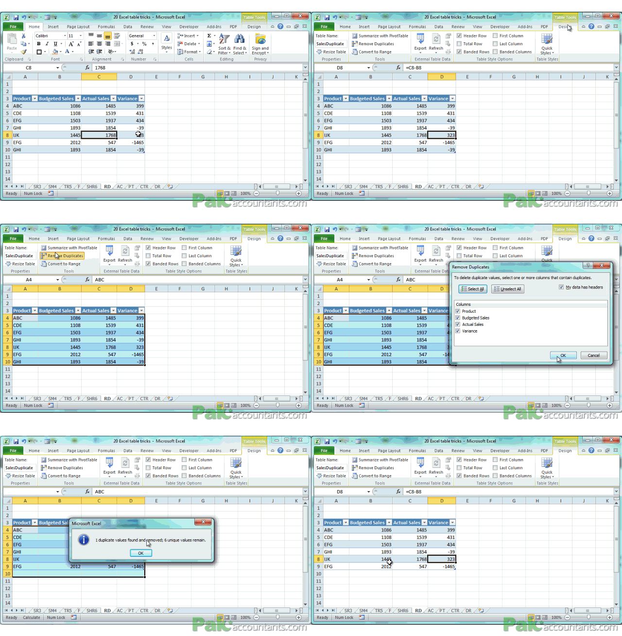
Excel Table Trick # 9. Hide/Show headers
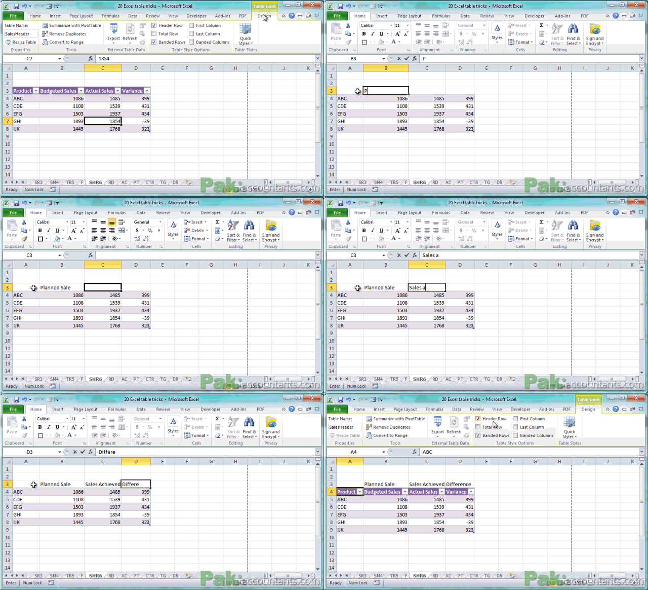
Don’t want to show table headers. Well you don’t have to delete that row. You can simply hide it by going to contextual tab>Table style options group> Uncheck Header Row. This will not only disappear in the worksheet but also from the print. Once hidden you can give another headers if you like with ease without affecting the actual table headers.
Excel Table Trick # 10. Covert table back to normal range
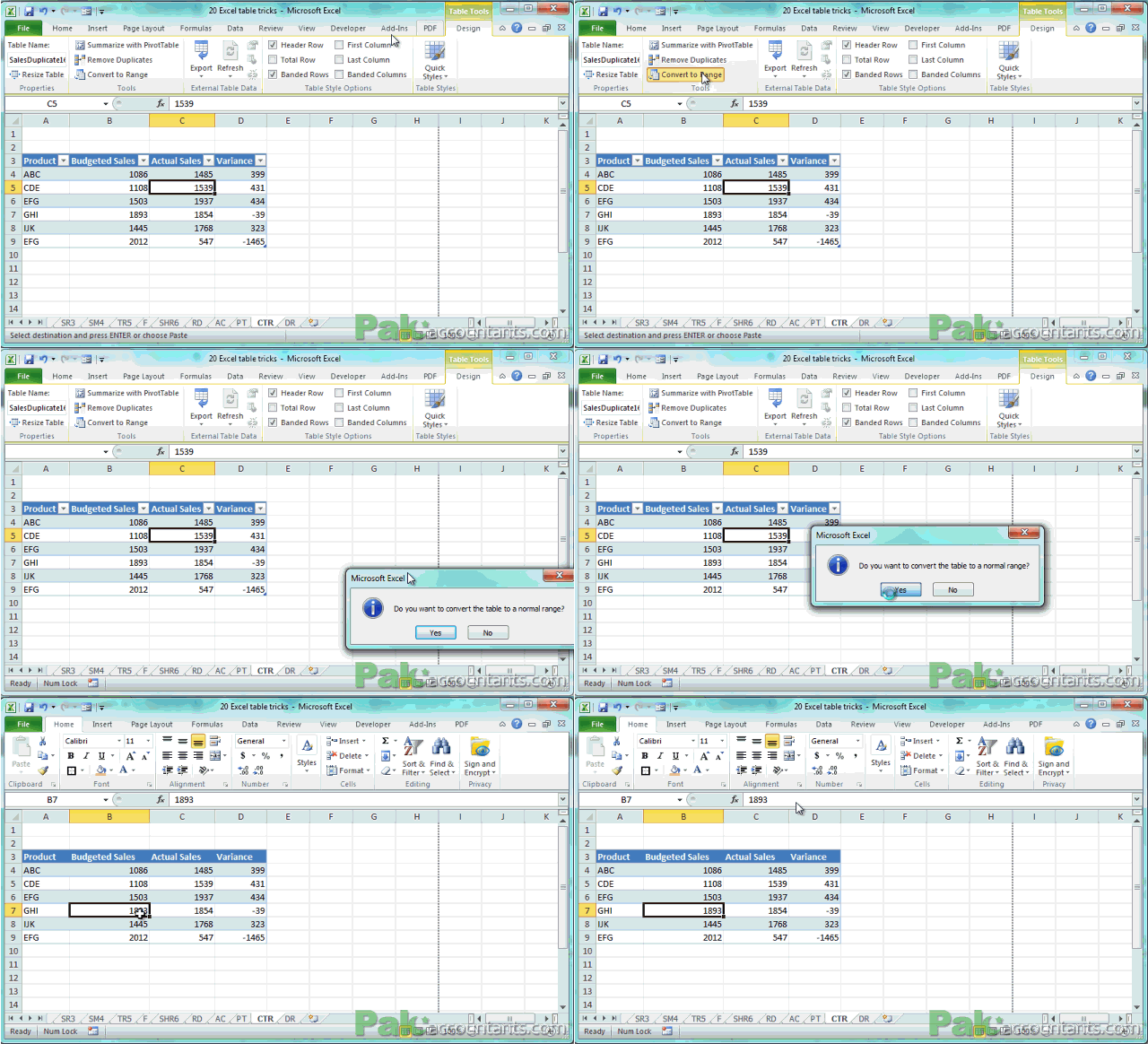
Not into tables anymore? Or for some reason you want to get rid of tables you can always get things done and click “convert to range” button in the tools group under table’s contextual tab. This will remove the table feature in a way that it dodges eyes. Colors and quick styling will be in place just tables have been drawn. You might need to do it if you want to export file to older versions of Excel as table feature comes in 2007 version of excel.
Excel Table Trick # 11. Selection made easy
You cannot escape selection in excel and its like addiction. But as usual addictions comes with problem and you might find selecting long data painful well tables come with selection features as well.
Selection with mouse
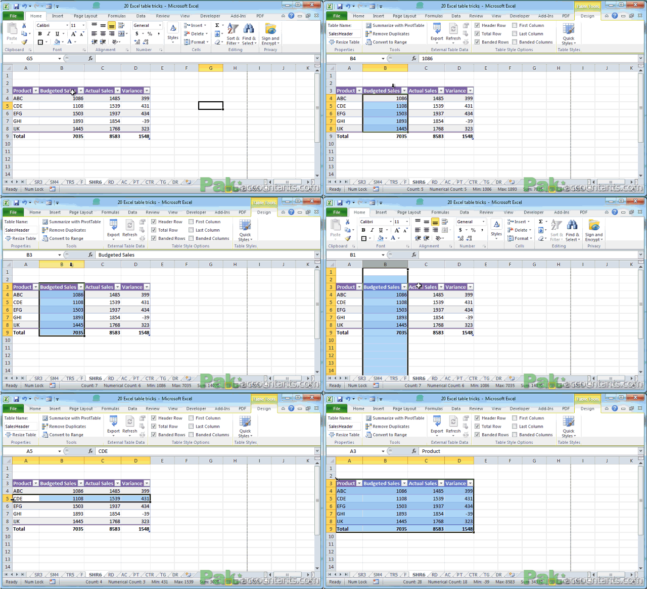
To select the whole column of table just move pointer to the edge of table (not out of table) and it will turn black in color pointing downwards, click once and it will select the whole data inside column. Click twice and it will select the header and total row as well.
If you move cursor far out of table it will help you select the whole column of the worksheet.
To select table’s row simply move the mouse cursor to the edge of that row but not out of table and it will turn black pointing right. Click once to select the table’s row. If you move cursor far left out of the table it will help you select the entire row of worksheet.
You can select whole table at once by moving mouse pointer at the top left corner of the table. Pointer will turn black pointing diagonally to bottom right corner of worksheet. Click once and whole table is selected.
You can also select multiple rows or columns by hover mouse pointer at the edge of table then click and drag to make multiple row/column selection.
Selection with keyboard
Having an active cell within the column of table you want to select press Ctrl+Spacebar. Hitting once will select the column data. Hitting twice will select the whole table column including header and total row. Hitting third time selects the whole column of worksheet.
To select the row of table, have active cell within that row and hit Shift+Spacebar. Hitting this combo once selects table row, hitting twice will select the entire row of worksheet.
To Select multiple column or rows then after selecting a single column or row as stated above press and hold Shift key and use directional keys to extend the selection
To select the entire data inside table hit Ctrl+A or Ctrl+Shift+Spacebar once. Hitting any of the two twice will select the entire table including headers and total row. Hitting any of the two thrice will select the whole worksheet.
Excel Table Trick # 12. Table headers replace excel’s default column headers
Normally if you have headers in first row and data is extended long down the rows then scroll down will hide the header row and its a bit frustrating as you have to scroll up and down back and forth to know what column holds what data. Possible solutions are freeze panes or split window.
But with tables you don’t have to do this. Having an active cell within table if you scroll down and just when headers are about to get disappear in the fold, headers replace the default column letters with Table’s headers. Such a clever little feature!
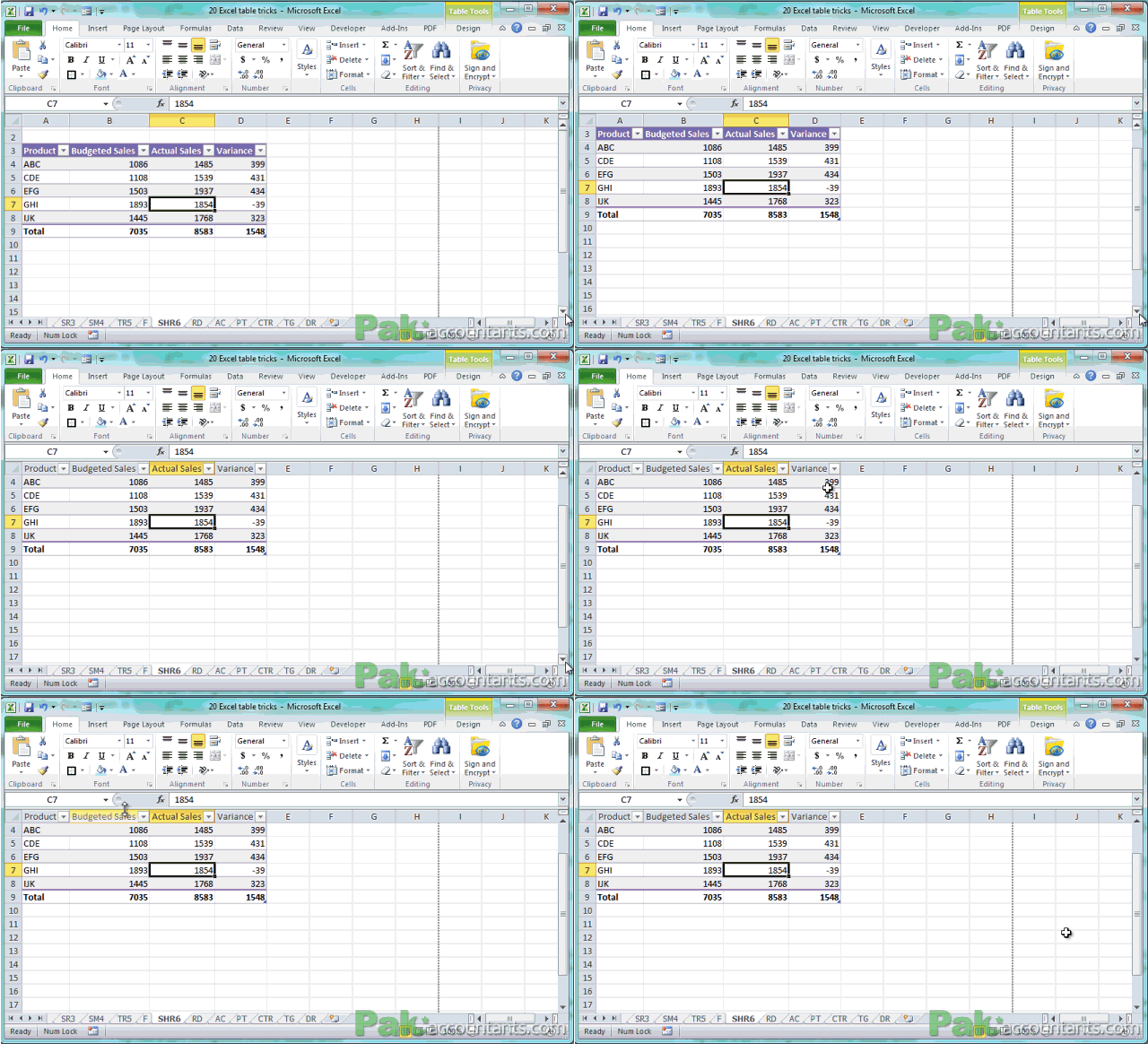
Excel Table Trick # 13. Get a new navigation system inside table
Normally when you press a Tab key it moves to the right. Same is the case in table. However, once you reach the last column of the table press the tab key again and it will go the next row. Similarly once you reach the last cell of last row, pressing tab key again will insert a new row in the table.
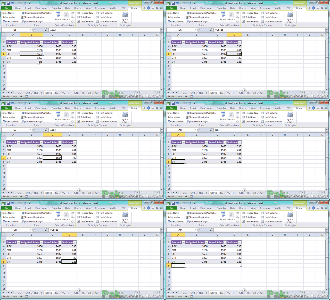
Excel Table Trick # 14. Drag and drop table easily without worrying about change in cell reference
With normal data ranges even you can move them easily by selecting and dragging-dropping them. However, if formula is dependent on such ranges then most probably it will break. However, with tables you do not have to worry if you have to move tables within worksheet anywhere if you are using structured references.
To move data simply move to the edge of table at the right or bottom of table and pointer will turn into four-point cursor click and hold to drag the table and move to other place. And if you have not noticed you don’t have to select the table first to move it. Saved you a shortcut key even 😀
Following animation makes it clear.
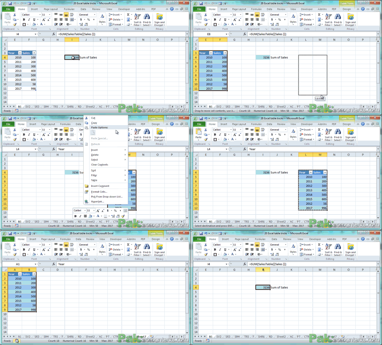
Notice that formula to sum the yearly sales is:
=SUM(SalesTable[[Sales]])
Now even if you move the table within worksheet anywhere or even to another worksheet altogether this formula won’t break. The reason is that structure is worksheet and cell address independent. We have named the table in the formula and particular column now wherever this table is formula will work without a hitch.
Excel Table Trick # 15. Print table separately
Want just the table? Well you might already know how to print selected data using print area option. But table saves you that time as right in the backstage view when you go for print you can choose to print the selected table and only that will be printed for you skipping other parts of worksheet/workbook.
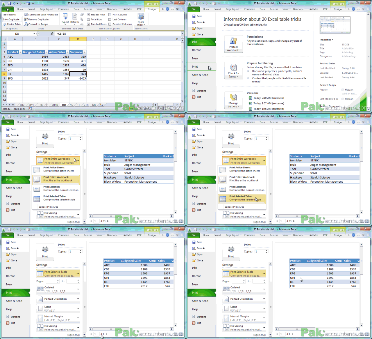
Excel Table Trick # 16. Export table data
With a sharpoint server in place you can directly connect the table’s data easily. And once connected you can modify table to have its effect being rendered on run time basis on the other side saving you the trouble of exporting data every time. Do it once and forget it!
Excel Table Trick # 17. Special formatting for first and last column if you want
Have a specific data in first and last column of table and want to format it differently. Check and done! Turn to contextual tab>Table style options tab>Check First and last column to have them formatted differently like change font size, color, weight, cell color, border etc.

Excel Table Trick # 18. Automatic extension of table as data grows
In tables if you are entering data and reach the end of table then just hit tab key and active cell will move to the first cell of next row extending the table formatting automatically and you don’t have to do any of the styling or writing formula as table will manage this for you on its own.

Excel Table Trick # 19. Help you create dynamic named ranges easily
We have discussed this great ability of table in Pivot table but exactly under its name. Actually table is a dynamic data structure that grows and shrinks with the data. This way you can easily apply functions without worrying about the data falling out of range and getting #REF! errors. Remember to harness this power we have to use structured references as structured reference is independent of cell references in a way that it is dynamic.
For example if you create data validation lists from named ranges then they are more of static in nature and if later your data grows then list won’t update with it. Following animation explains it:
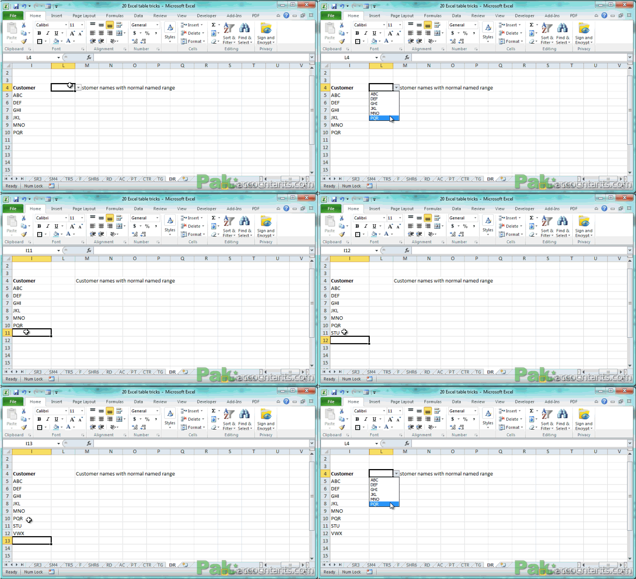
But if the same is done using tables then you get dynamic named ranges and your data validation list gets updated if your data grows. Following animation makes it even clear:
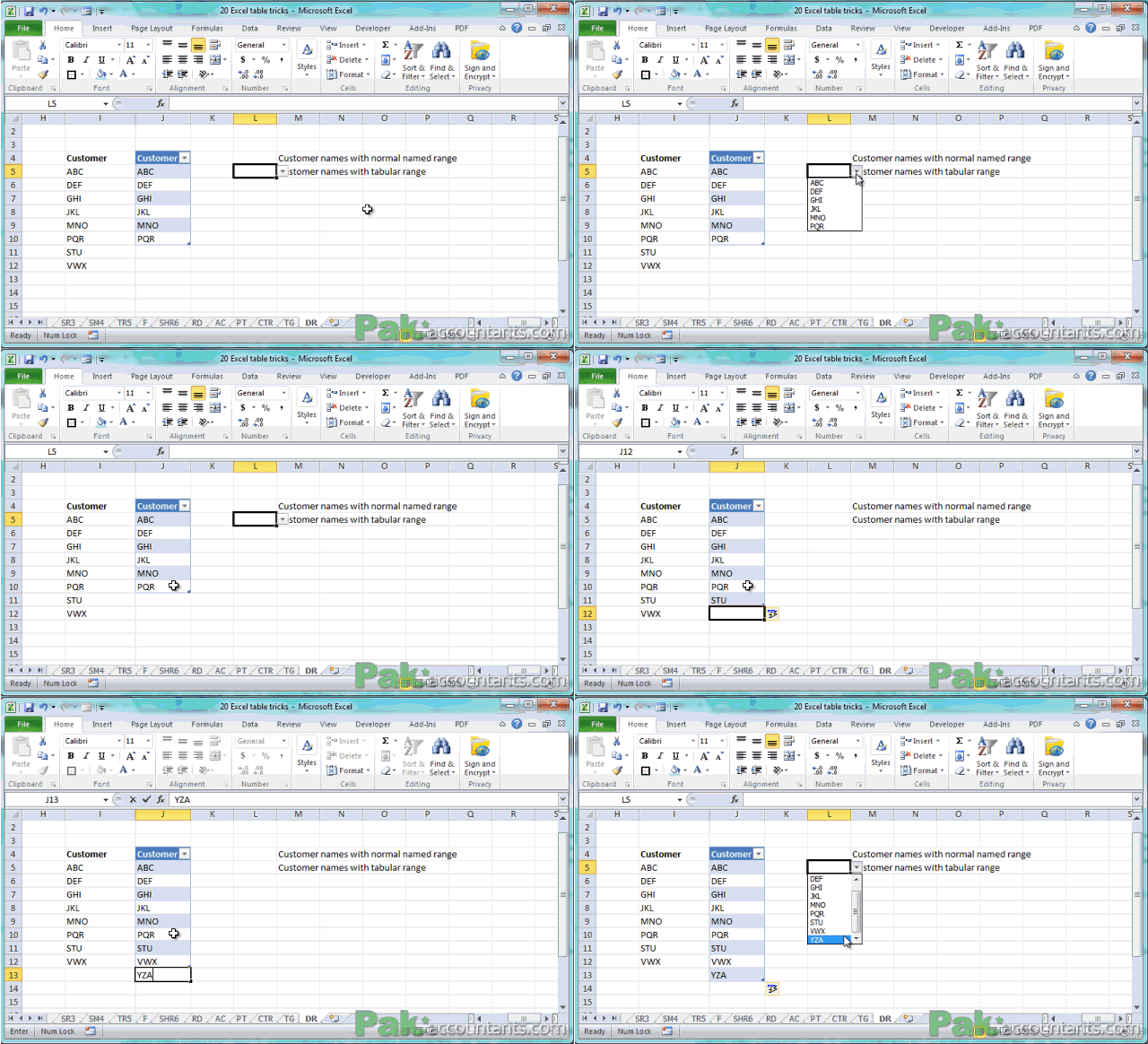
To learn how to make data validation lists from tables check out our data validation tips and tutorials
Excel Table Trick # 20. Making turbo charged going on rocket fuel! Table to Pivot table
If table are the big thing you learnt then hold on until you learn table’s elder brother Pivot tables. With normal range you might have to perform some preliminary steps to prepare the data for pivot table purposes but with data arranged in tables you don’t have to do much.
But the best part is that if your pivot table is based on table then just by updating table, your pivot results will also update. This does not happen in case of normal range based pivot table. For instance if data grows pivot report will not include new results but with table at the back end its just taking things to next level. Include the new data and refresh pivot table and you have the new pivot table including the new data. This saves tons of time as you don’t have to reconstruct pivot table from scratch. 🙂 Excellent!
Following steps help you make pivot table from tables and then understanding how pivot table gets updated if new data is included:
Step 1: Make sure AC tab is active. You can see a large table on this sheet.
Step 2: Having a active cell within the table click contextual tab. In Tools group click Summarize with Pivot Table button.
Step 3: Excel will insert a new worksheet automatically to let you create pivot table. From the pivot table field list drag the items from the list to four squares below as follows:
- Drag year to Report filter
- Drag Products to column label
- Drag Sales person to row label
- Drag Total to Values
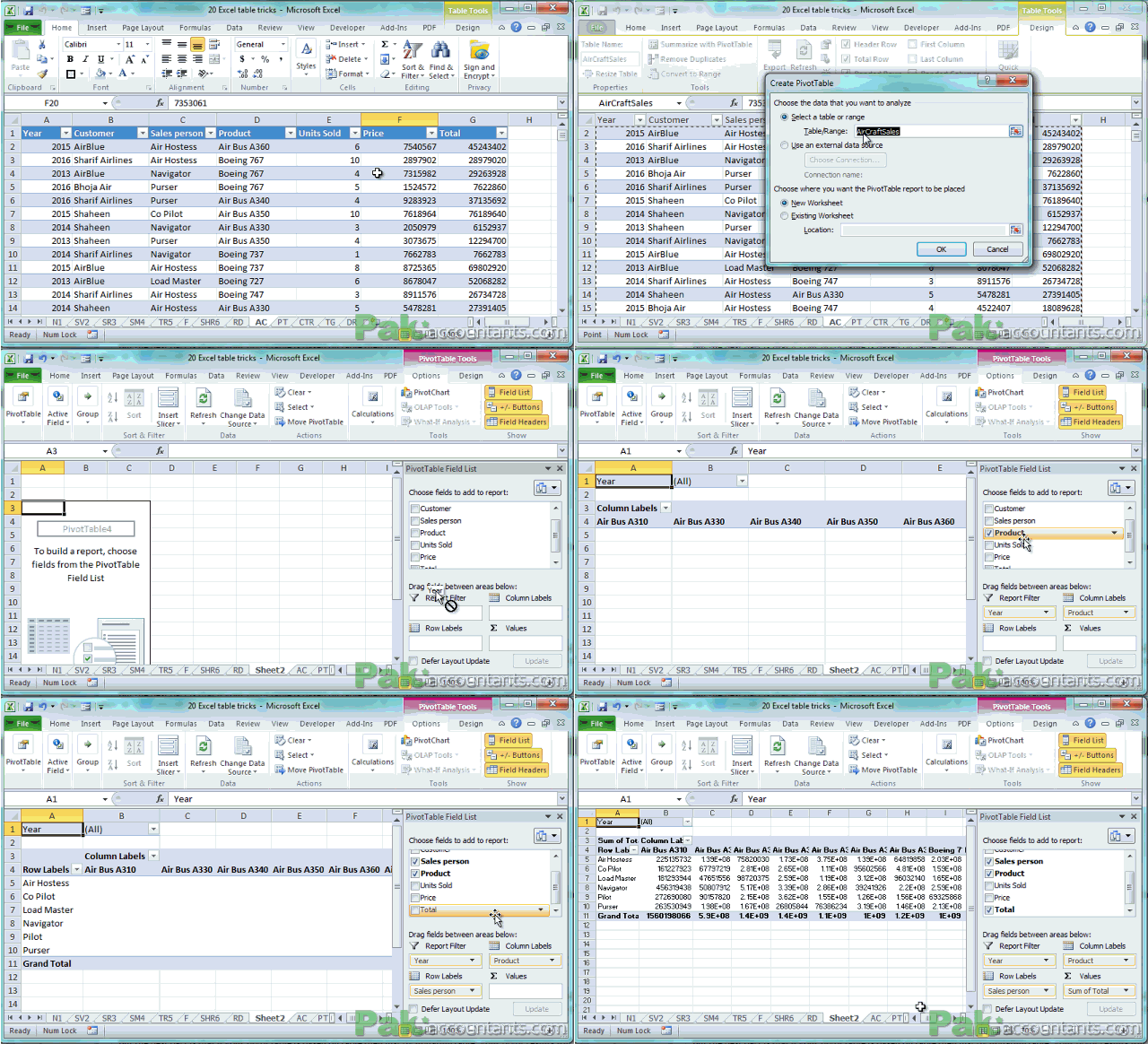
Now you have the pivot table done for you giving you the information how much revenue is generated by each sales person in each product.
But if you like to know how much sales are made by each sales person to each customer, you can find out that as well. This is what pivot tables are; swift easy results out of numbers. To get this information following these steps:
Step 1: Click anywhere inside pivot table so that pivot table field list appear again.
Step 2: From the column label box below, drag the products out of it by clicking and dragging it out. This will remove products.
Step 3: Drag customers from the list and drop it in the column label box.
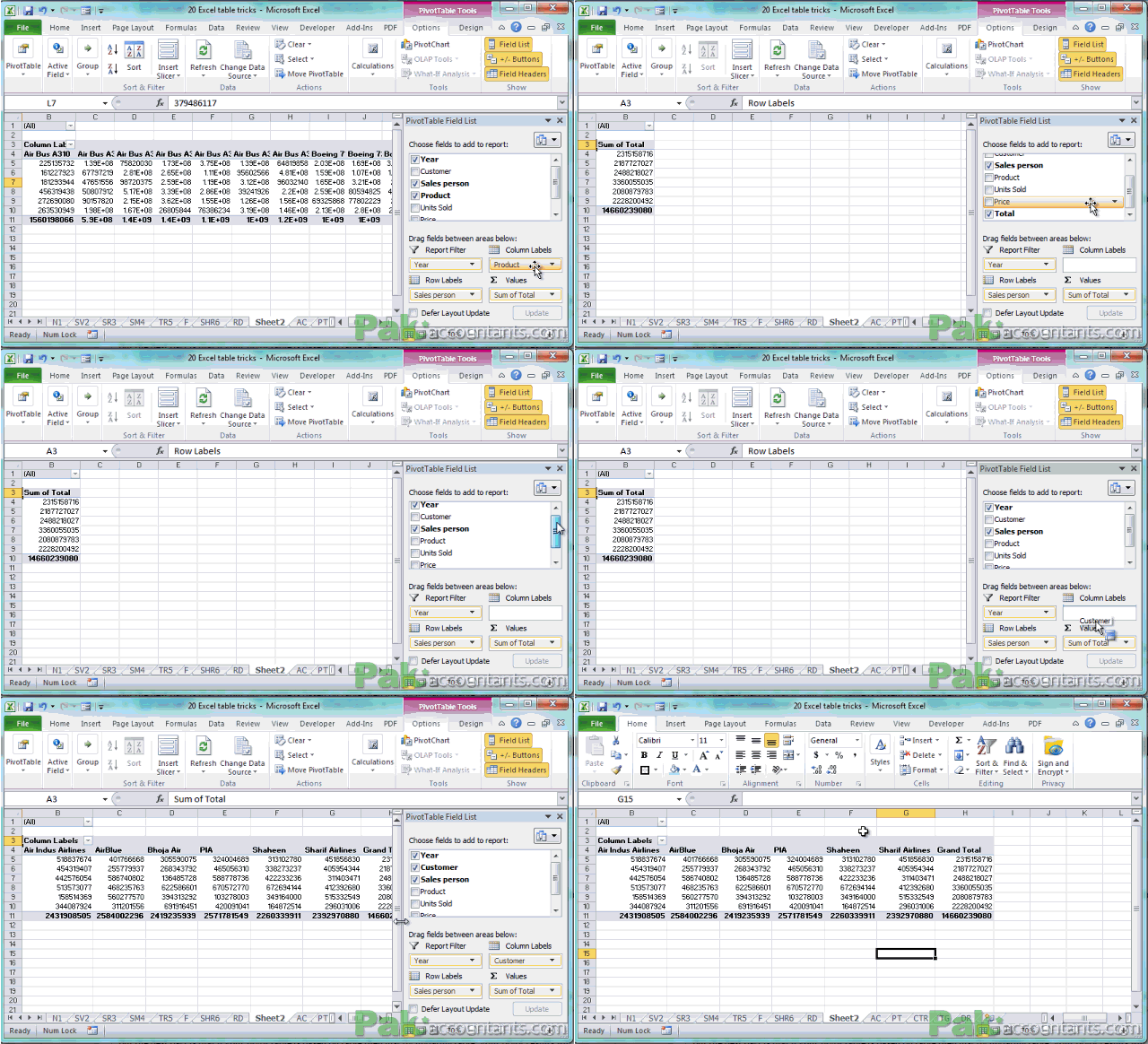
Your required report is ready giving you information about how much each sales person made from each customer.
But what if our sales data grows? Do we have to make pivot table again? Well if your pivot table was based on normal range then this might have been the case. But as our pivot table is based on table, therefore if you add new data to it and refresh the pivot table, the new data gets included automatically saving you the whole process of reconstructing the pivot table from scratch
Watch following animation where we included two new records with customers Lufthansa and Kamra, sales person: Hasaan selling Jango air crafts. Once refreshed pivot table includes newly entered data. FAN TABLE OUS!

Excel Table Trick # 21. Get a tailor made data entry form for each table independently – Unearth!
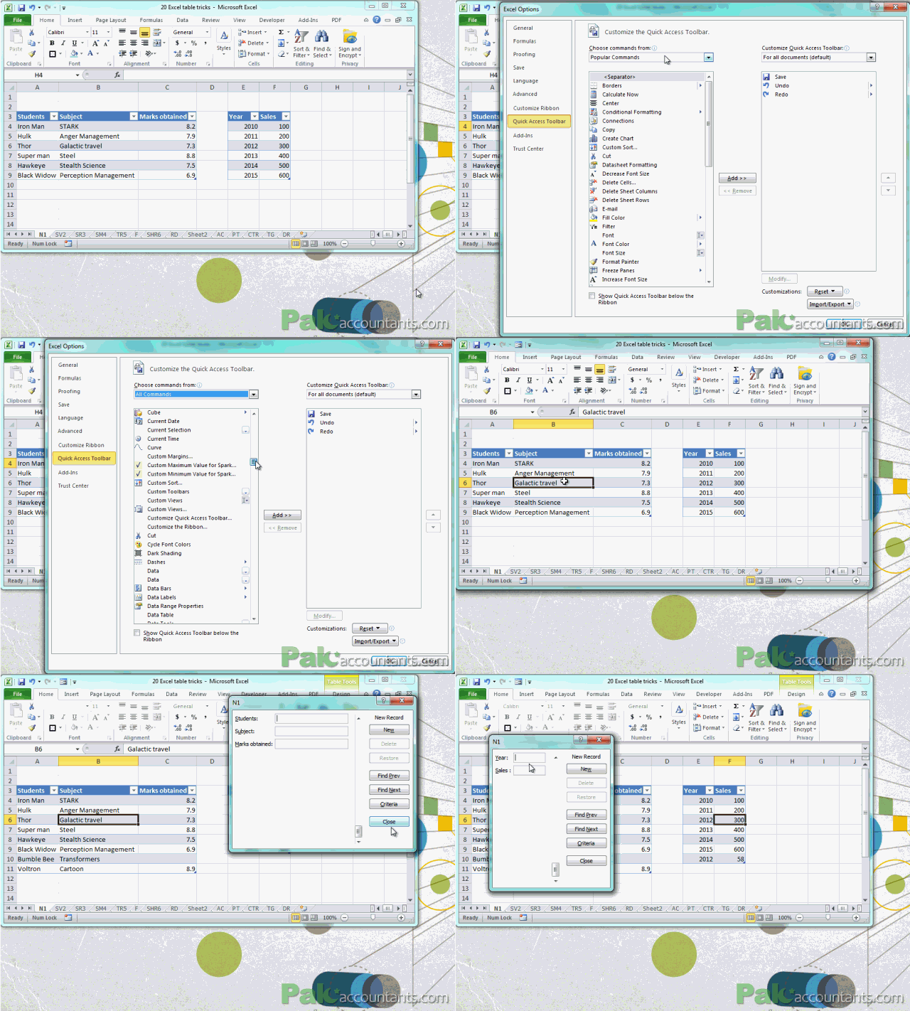
For those who don’t know it will be like finding a hidden treasure. Excel forms feature is not visible and accessible from the ribbon. So a lot of excel beginners don’t know of its existence. Excel forms is one way of making data entry easy and smooth and formal in looks. Every table comes with its own individual form by default and can be used to populate table.
To access forms follow these steps:
Step 1: Right click on quick access tool bar (yes that little button bar you thought is no better than saving or undo button is a complete package). From the menu select “Customize quick access toolbar”
Step 2: Excel options window will open. From the “Choose commands from” drop-down menu select “All commands”
Step 3: Scroll waaaay down to find “Form…” Don’t worry list is alphabetically ordered so finding it won’t be that hard. Once found click Add button. And finally click OK at the bottom of excel options window.
There you have forms button in your quick access toolbar. Have the active cell within table and click the button. And a form will appear to let you enter data in the table. Smoooth!
Loved the tricks? Pin it!


Leave a Comment