Using Excel Custom Number Formatting as Data Validation Tool

 Excel custom number formatting feature is immensely powerful. From hiding things to formatting telephone numbers correctly, to changing colours to use them to insert symbols in data or chart, it is definitely of great use.

Today we are looking at this tool for yet another purpose which is kind of odd but still works!

Data entry jobs are quite a nuisance as they are prone to human errors and even a careful data puncher may end up making mistakes. To assist such users we use data validation features that intimate user if a wrong data is entered. And on intimation user can make correction.

Suppose you have a form in which you are entering information about the user and one field is about telephone or contact number. Now contact number cannot be negative or text and also it must have certain minimum numbers. We can use custom number formatting feature to do the data validation task.

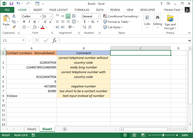
Lets you have the following data entered for contact numbers and in column B we have the comments:

Definitely there are some mistakes, some numbers are in negatives, one cell has text instead of number, some are incomplete etc. This is what happens when you are not having data validation active and thus you are not intimated that you have entered a wrong data.

Here in our example the data set is really small and so we can find the problem easily but situation where hundreds of contact numbers are entered on daily basis, things get really difficult. So we need a solution that prompt us that wrong data is entered as and when it is entered instead of looking for wrong data after the whole input is done.

Select cell C2 through C8 and hit Ctrl+1. This will invoke format cell dialogue box with number tab active. In the left side click Custom and the in the type field put this code:

[<=999999999]"Can't be less than 10 digits OR negative";[>999999999999]"Number can't be this long"; 00-000-0000; @ - "Can't be a telephone number"

This code has several parts divided with colon “;” mark and what each means is explained as follows:

[<=999999999]”Can’t be less than 10 digits OR negative”
This part of code is checking if the numbers are entered are smaller than 10 digits then it will display the message “Can’t be less than 10 digits or negative”

[>999999999999]”Number can’t be this long”
This part of the code is checking if the number entered is longer than 12 digits than again its wrong and there might be a repetition of digits and thus displays a message “Number can’t be this long”

00-000-0000
This is the code for correct contact numbers entered. And is telling the Excel to format the telephone numbers in this way.

@ – “Can’t be a telephone number” 
This part of the code will work if text is entered instead of a number in the cell in which case Excel will display that text and the message that it “Can’t be a telephone number”

Now try to put the same numbers in column C as they are in column A. For example type in the contact number as we have in cell A2 in cell C2, A3 in C3 and so on and you will see Excel doing its work intimating you if wrong data is entered!

SuuuuWWEEEEEEET!!!! 🙂 I love custom number formatting.

Check out more of our tutorials where we can see custom number formatting in action  by visiting this page and if you ideas to make this trick even better then do share in the comment section below.