Transpose Data in Excel: Shift Columns to Rows or Rows to Columns – 5 Methods Explained

In Excel one can easily convert data columns to rows or multiple data rows to columns which is technically named transpose.

What is Transpose?

In Excel switching or rotating columns to rows or rows to columns is called Transposing the data.

And this actually shifts the dimensions of data and along with it definitely the address of different data bits will also change. Therefore, if you are into transposing your data, do it with caution as if you shift the data the dependent cells might miscalculate the figures.

Love reading about Excel? Subscribe my youtube channel dedicated to Excel.

[vc_btn title=”Subscribe” style=”custom” custom_background=”#ff0000″ custom_text=”#ffffff” size=”lg” align=”right” i_icon_fontawesome=”fa fa-youtube-play” add_icon=”true” link=”url:https%3A%2F%2Fgoo.gl%2Fx16inH||target:%20_blank|”]

Many already know how to do this. But for those who don’t this one minute Excel tutorial is for them. By the way, yes! you can use pivot tables to shift rows as columns. To learn how to make pivot tables read this readers’ favourite tutorial. And most probably you will figure out the way how rows are shifted as columns using pivot tables.

We have several ways to switch or rotate Excel data columns to rows or vice versa to accomplish this task. Following are the transpose methods we are discussing today in which few involve converting columns to rows using Excel formulas:

Use Paste Special
Use TRANSPOSE function
Use INDIRECT function
Use INDEX function
Use Paste Special + Common Sense

Method 1: Convert columns to rows using Paste Special

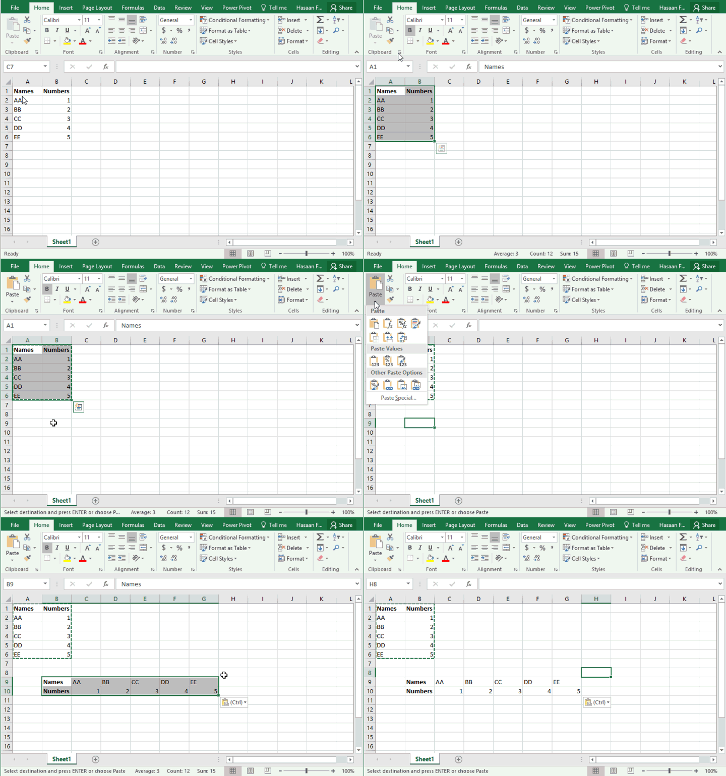
Copying and Pasting is one great thing happened to PC. With Paste Special it really went miles ahead. In Excel you can copy a data and then using paste special functionality you can twist, rotate, manipulate, process and do other things with the data very easily including Transpose i.e. flipping columns to rows or rows to columns. To do this following steps will help:

Step 1: Select the data that you want to transpose and copy it using the copy button or with Ctrl+C shortcut.

Step 2: Go to the cell where you want the data to paste. And go to Home tab > clip board group > click the drop down button just under paste button > select:

under paste sub-group click transpose button that comes with this icon; OR
Select paste special. This will open the paste special dialogue from which check the transpose checkbox and click OK button

Your data will be transposed instantly. Told ya! it is easy!

Method 2: TRANSPOSE Function to switch columns to rows or vice versa

Yes there is a function that can do the somersault called TRANSPOSE. The use of this function is a little tricky and requires knowing more than pressing TAB so follow the steps closely.

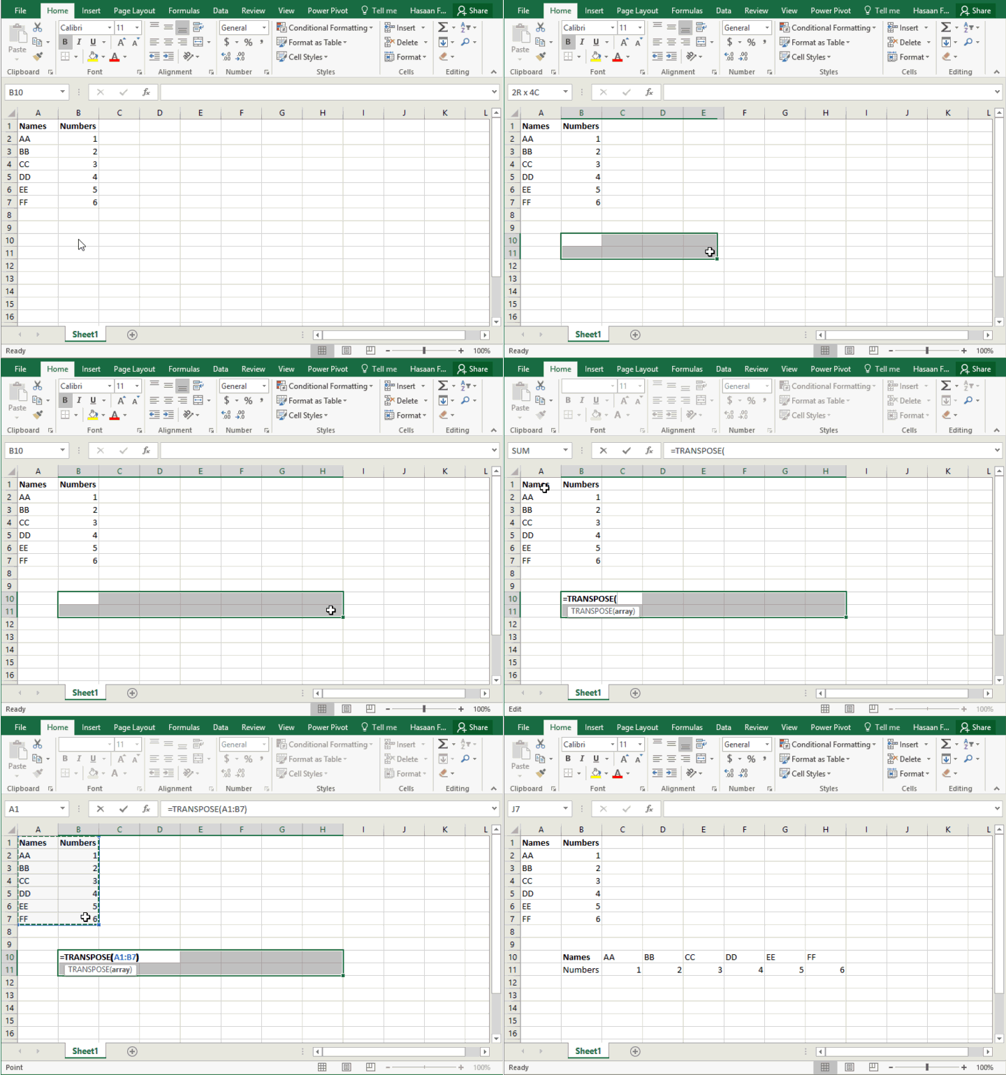
IMPORTANT: Determine the rows and columns of your data. For example you have 2 columns and 7 rows. Once you transpose the data it will be 2 rows and 7 columns.

Step 1: Determine the rows and columns of data. In our case it is 7 rows and 2 columns

Step 2: Select a vacant region in the worksheet which is 2 rows deep and 7 columns wide.

Step 3: Press F2 key to enter edit mode while the region still selected.

Step 4: Write TRANSPOSE function following the equal sign and enter the data range that you want to transpose

Step 5: Hit CTRL+SHIFT+ENTER. Yes! Not just Enter key but Ctrl+Shift+Enter as this is an array formula

TANGO! Your data is transposed!

Benefit of TRANSPOSE Function

The best thing with using TRANSPOSE function is that if you change the values in the source range then transposed range will also change accordingly. So basically it is a live-transposed-range of the source-range.

But as this is an array function this is very much dependent on the source and if you try to change anything this tends to break. Therefore, even if it is good for many reasons, it is hard go by in many situations. So follow along to learn some more easier to go tricks to get the data transposed in Excel.

Method 3: TRANSPOSE Using INDIRECT function

INDIRECT function was introduced in one of my favourite article some time back in which we learned how to build a reference to worksheet based on cell value. I must confess that I used to think INDIRECT has very little use but this little function can prove tremendous help.

Today we will look at another use of INDIRECT function i.e. to transpose the data. However, if you use this function the treatment for column to row shift is a little different from row to column shift. So I will explain both one by one.

Transpose – Column to Row using INDIRECT

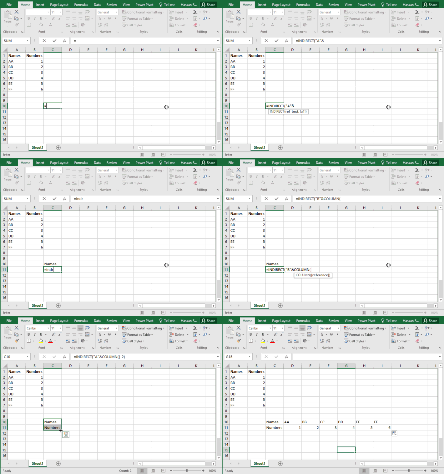
Suppose our data is based on 2 columns A and B and 7 rows from 1 to 7.

The data of column A has address like A1, A2, A3,…. A7. In this A is constant whereas due to additional rows we have increasing numbers from 1 to 7. If you understand up to this, you will understand what we are about to learn.

Lets say you want to put the transposed data starting at cell C10. I will put this formula in cell C10 and press Enter key:

=INDIRECT(“A”&COLUMN()-2)

And this formula in C11 and press Enter:

=INDIRECT(“B”&COLUMN()-2)

Now select these two cells and drag the fill handle across to column I. So there you have the data transposed. But lets understand what formula is actually doing.

Understanding INDIRECT approach to TRANSPOSE

As told earlier Indirect formula helps in converting text strings to cell references. COLUMN function actually gives us the number of column in which the formula is entered. For example if you put =COLUMN in any cell of column A it will give the value of 1 as it is first column. Similarly if you put the COLUMN function in any cell of column I, it will return 9 as it is 9th column.

So with the column function we were able to incremental numbers as we drag the formula across columns. But as we inserted the formula in third column and the not first column so it would have returned 3 in which case the first address to be fetched would have been A3. But we want the values from first cell of column A therefore we had to insert “-2”. This way we got 1, 2, 3 and not 3, 4, 5

So the formula: =INDIRECT(“A”&COLUMN()-2)

In the above formula “A” is provided as text string which is joined (concatenated) using “&” with the values generated through COLUMN function. And thus successfully built the cell references.

Now if you change the values in source range the transposed range will also change. But it is much more flexible as it won’t break if you change one item in transposed range manually.

Transpose – Rows to Columns using INDIRECT

~~Using the same technique learnt above, we can transpose the data from rows to columns. But in this case you will use ROWS() function instead of COLUMNS to work correctly.~~

As you are converting rows to columns therefore you will be going down the rows and thus you require number increments as rows are jumped. So simply adjust the formula as per your needs and use ROW instead of COLUMN and it will do the rest for you.

No you can’t simply replace the COLUMN function with ROW function as mentioned above to convert the rows back to columns. Instead you will have to use the combination of INDIRECT, ADDRESS and ROW function.

In my case to transpose first row to column I used the formula: =INDIRECT(ADDRESS(10,ROW()-11))

Whereas to convert the second row to column I used this formula: =INDIRECT(ADDRESS(11,ROW()-11))

Method 4: TRANSPOSE using INDEX functions

Using the technique learnt to transpose columns to rows above. You can use INDEX function if building reference is difficult for you and you still have your head spinning.

INDEX function is one great addition to Excel functions and formulas repository. Lets have a look at the syntax of INDEX very briefly so that we understand how can we use it to transpose the data.

INDEX(array, row_num, [column_num])

array: the range, in our case it is the range we want to transpose

row_num: the row number. In this function we have mention row number to help it fetch the value

[column_num]: this is the optional argument. If not mentioned the column number doesn’t change and it will be the same in which function is applied. But today we need this option badly!

Transposing Rows to Columns using INDEX function

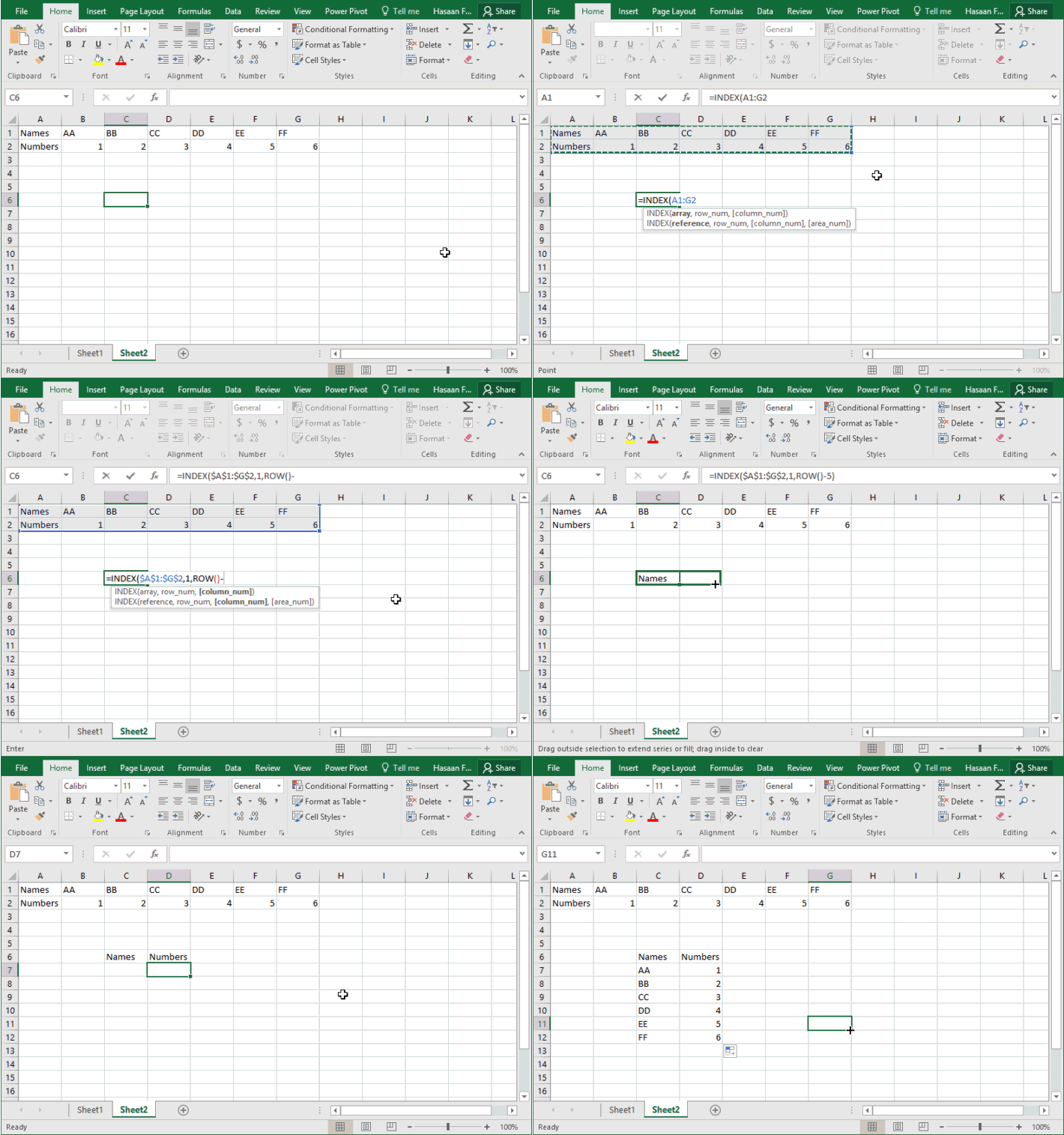
Suppose our data is arranged from cell A1 to G2. Two rows and seven columns in other words. So if we transpose the data we will have 2 columns and 7 rows.

To transpose the data arranged in a row to column go to the cell from where you want the data to start. I selected cell C6 and D6 and put theses formula:

Cell C6: =INDEX($A$1:$G$2,1,ROW()-5)

Cell D6: =INDEX($A$1:$G$2,2,ROW()-5)

Select both cells and drag the fill handle down to next six rows i.e. row 12. And you will get the data transposed from rows to columns.

Understanding the formula

Lets take some time to understand the mechanics of this formula. The formula we applied in cell C6 is as follows:

=INDEX($A$1:$G$2,1,ROW()-5)

array: [$A$1:$G$2] – this is the range that we want to transpose. The reference is made absolute so that as we drag the formula this array stays static and does not change.

row_num: [1] – this represent the first row of the data and we mentioned it so that INDEX function recognize that we want it to fetch the values only from row 1 of selected array i.e. $A$1:$G$2.

column_num: [ROW()-5] – Our data A, B, C, … G is in one row but across 7 columns. That means the address of:

value A is first row-first column
value B is first row-second column
value C is first row-third column; and so on…

So as we drag the formula down, we want the formula to get the values from 1st, 2nd, 3rd, 4th, 5th, 6th and 7th column. To do this we have to tell the column number. Now one way is to mention column number manually every time we put the INDEX function in next cell so that it fetches the right value.

But to automate the process of feeding column numbers to the function, I used ROW() function as the argument of column number (column_num). And as I drag the fill handle down, the ROW function will churn out row numbers inside the formula.

ROW function gives the row number. Now as I have put the INDEX function cell C6 the ROW function will tell that ROW number is 6. But we want it to be 1 as I want to fetch the values from the first column of the selected array. That is the reason we have “-5” following ROW() inside the formula. So it reduces the numbers generated by ROW function by 5 and this it will give 1, 2, 3, … 7.

Transposing Columns to Rows using INDEX function

Once you understand how INDEX function has fetched the values in above situation. Its easy to understand how to tackle the data which is arranged in columnar form and we want it to shift in rows.

For this we will make two changes:

for row_num: now we will use COLUMN() function generate numbers so that as we drag the formula towards right the row number will get updated because we are jumping across columns and thus COLUMN function will fetch the column number. Adjust the value generated by column number by adding or subtracting constants so that you get the desired result.

for column_num: mention 1 or 2 depending on the column within the selected array from which you want the values fetched.

Example

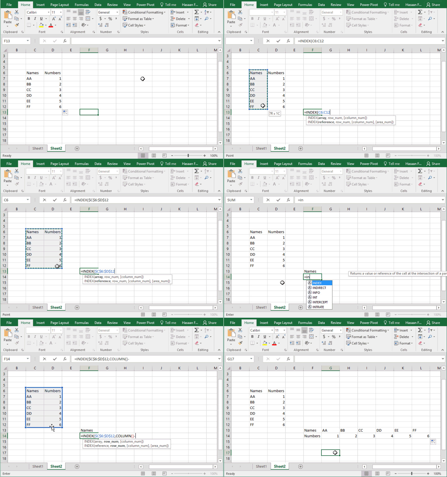
For example my data is based in 2 columns 7 rows and is housed in column C and D starting at Row 6.

I want the data transposed in rows 13 and 14 in column F. Therefore I put these formula:

cell F13:

=INDEX($C$6:$D$12,COLUMN()-5,1)

cell F14:

=INDEX($C$6:$D$12,COLUMN()-5,2)

Select both cells and drag to the right until column L

Method 5: Paste Special + Common Sense = Paste Ultimate!

We saw TRANSPOSE function went ahead of Paste Special as it was not only able push columns as rows (transpose) but were also live as transposed range was able to update as source change. We fixed some of the TRANSPOSE nuisances through INDIRECT approach. But writing formula and then dragging the range takes time.

But can we get TRANSPOSE like result using paste special? The answer is yes!

Paste Link

To get the live feed of source range we can use Paste Special’s inhouse capability called Paste link. Paste link pastes the cell references and not the values in cell and if source data changes, the linked cell will also change.

However, for unknown reasons, if you try to transpose and paste link at the same time Excel does not allow that i.e. you can either transpose or paste link. In other words, if you click Paste Link button with transpose option checked, the moment you select transpose option the paste link button gets disabled.

To get around this misery we took help of our Agent-X named common sense. Follow along!

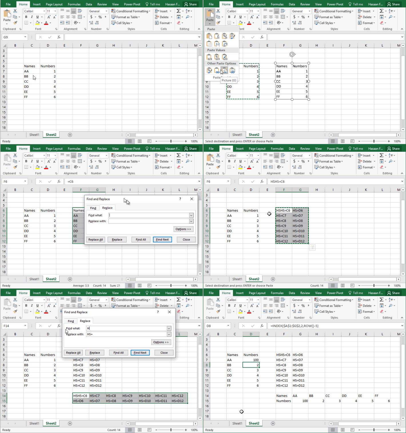
Step 1: Copy the range and go to any vacant space in the same worksheet.

Step 2: Hit Alt+Ctrl+V to invoke paste special dialogue box and hit the button paste link. This will paste NOT the cell values but the cell references of the range you copied.

Step 3: Select the range you just pasted and hit Ctrl+H. This will bring up the REPLACE dialogue.

Step 4: In ‘Find what’ field mention equal sign i.e. “=” (without quotes) and in replace with field mention “HS=” and hit Replace ALL button. This will actually convert the formula into text as you have just replaced the equal sign with HS=

Step 5: Copy the range again and now go to the place where you want to put the transposed range. Hit Alt+Ctrl+V to bring the paste special dialogue box. Select the Transpose option and click OK. This will effectively transpose the data.

Step 6: To revert the formulas back in place so that you get the correct values in place from the source range. Hit Ctrl+H again. This time in Find what field put HS= and in replace with mention =. Hit Replace ALL button.