Running Totals and Running Balance with Excel Pivot Tables – How To

Last time when I discussed how to do running totals and running balance using Excel many different ways were discussed but one was left for today which is doing running totals and running balance using Pivot Tables in Excel. The reason was by that time we didn’t discussed how to make pivot tables. But as we have discussed it now and learned how to make pivot tables in Excel now we can learn this technique.

Those who are new to running total and running balance concept they can read simple explanation of it on this link. I have explained it with accounting perspective.

Download Excel Tutorial Workbook

To understand better and to apply the techniques and tips learned in this how-to tutorial download this excel workbook and open this file in your Excel program

Running Totals with Pivot Tables – Three to Glee!

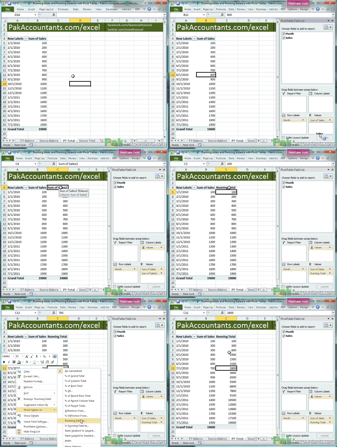
Open up the file you downloaded. In the Source-Total worksheet you have the data for which you like to calculate running total. PT-Total contains the pivot table already made for you. To learn how to make such a pivot table read a beginners’ guide on Pivot table.

Step 1: Click anywhere inside pivot table and field pane on the right will open. If task pane does not appear then go to Pivot Table Tools > Options > Show group > click Field list button.

Step 2: Click and drag the sales field and drop it under the already present “Sum of Sales”. New column in the pivot table will automatically gets added with the name “Sum of Sales2”. Click the header and replace the name with Running totals.

Step 3: Right click on any cell inside the newly added column (Running Totals) and from the context menu, move cursor over “Show value as” and from the submenu select “Running totals in”. A new dialogue box appear, click OK. You will get the running totals.

Following animation walks you through visually how to carry out these three steps:

Didn’t I told you Three to Glee? 🙂 Smack easy. No formulas, nothing new to be done. With pivot table in place its all a game of few clicks.

Running Balance with Pivot Tables

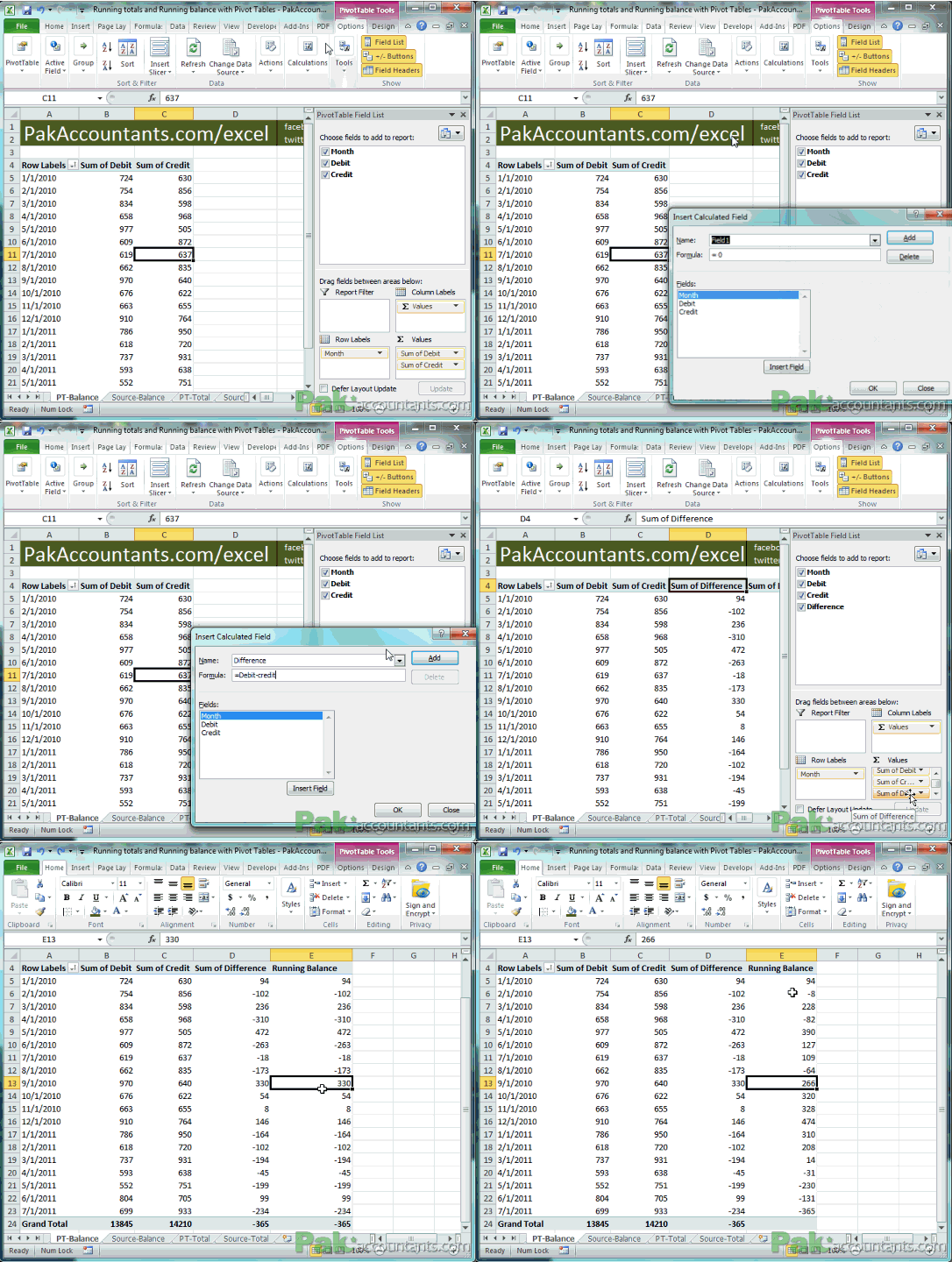
The source data is available on worksheet named Source-Balance. Activate worksheet named PT-Balance. Pivot table is already made for you. In this we have three columns; Months, Debit and Credit. We need running balance column so that we can assess the cash left after every transaction.

Step 1: Click anywhere inside pivot table and go to Pivot Tables > Options > in the calculations group click Fields, Items and Sets drop down and select calculated field.

Step 2: A new window opens. In the name field type Difference and in the formula type:

=Debit-Credit

Click Add button and then click OK to close the dialogue box. A new column with the name “Sum of Difference” will be added.

This way we will have line by line difference of debit and credit columns. But this gives us a balance of one line but not the running balance. To get that we will add another column to the pivot table that basically do the running total of “Difference” column we just added.

Step 3: Drag the Difference field from the field list and drop it in the values box in the last. A new column will be added with a default name of “Difference2”. Rename it as “Running Balance” by editing header of the column.

Step 4: Right click on any cell in the newly added “Running Balance” column > Show values as > Running total in. A new dialogue box appears. Click OK.

Watch the following animation to better understand the above four steps:

TADA!!!! Now you have the running balance column. Difference column is now not needed so simply uncheck it from the fields list pane on the right.

More Tutorials on Excel Pivot Tables

So my friend you have just excelled two steps forward on Excel’s advanced feature called Pivot Tables. We learned how to have running totals in pivot tables and also learned how to use calculated fields in pivot tables. There is a lot lot more you can do with calculated fields. The example I shared was a simple one. In future we are going to need this little feature of pivot table very often.

Liked it? Pin it!