Making Print Area dynamic in Excel feat. OFFSET function – How To

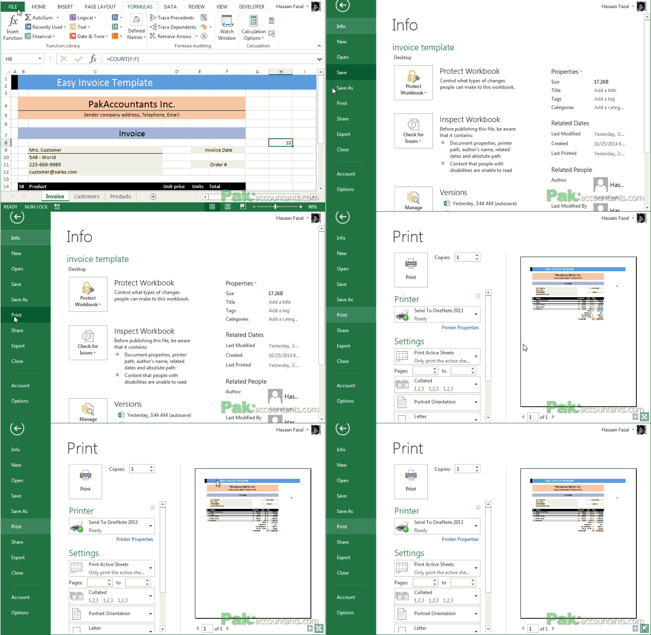
 Print area is simply the area which will be printed if you give a command either using Ctrl+P or going to File menu and Print.

Excel gives you the flexibility to set the print area. We have discussed this feature of Excel way back in time in this article: Excel Tutorial – Ctrl P is Power in Control (Printing). It has been one of the most read articles in our Excel repository. I totally recommend each and every reader to go through it as we learnt quite a bucket load of things we can do in Excel’s print options.

However, we are on a different mission. Have a look at this Invoice Template  V1.0 . Among other key benefits, one of them is dynamic print area or simply put print area changes as the data size changes. So, instead of having a fixed print area, if your invoice is big, print area will expand to incorporate all of the items, and if its small the print area will contract automatically. And today we will learn how to do it.

The idea behind dynamic print area is actually having dynamic named ranges.

Not many know that when you specify a print area in Excel, its actually a named range. And if it is a named range you can use all sorts of formula in it and thus it makes expanding/contracting print area.

Consider the following situation:

 As you can see it has big ugly blue heading “Easy Invoice Template” and after that the real deal starts. Now when I print it the problem is that ugly heading gets in the way.

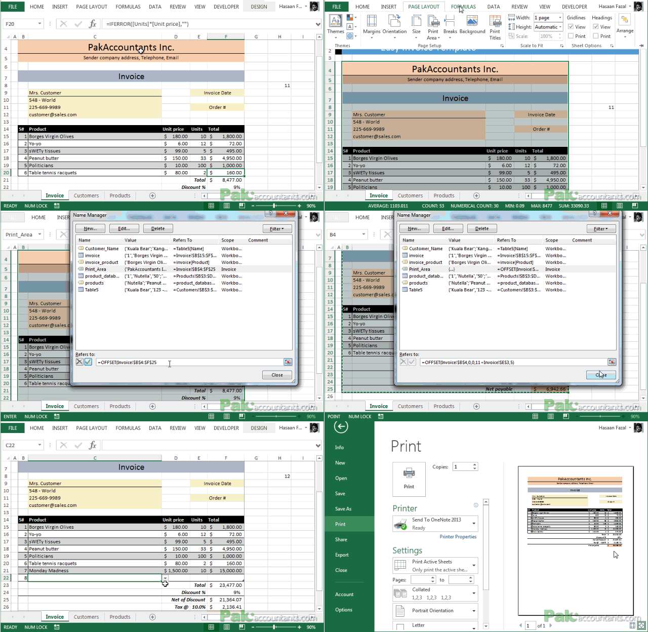
Now you might be thinking that you can select the print area and get rid of that heading above. But its a fix that needs to be fixed every time the invoice is updated. For example if we set print area by selecting cell range: =B4:F24 then it will stay fixed and if we insert more items the bottom will be cut out.

So need a way to make the print area dynamic so that it not only get rid of the top heading but also expands/contracts with the data.

So here is the trick:

1. Data is starting from Row 4
2. Until row 14 you have static data i.e. this is not going to expand or contract
3. From row 15 onwards you have the data that is dynamic and tends to change.

So from row 4 to 14 it makes 11 rows (including row 4) that are static and the rest are variable. So the print area is 11 rows + variable rows. As you can see that the part that varies is actually residing in column F. So if we can count the items in column F every time, we can work out the print area.

This is where our OFFSET function is going to help us.

First of all set the print area as normal. Just select whatever data you have and go to page layout tab > page setup group > print area drop down > set print area.

Now you have specified a print area. Go to Formula tab > defined names group > click names manager. This will open names manager box. Find the name “Print_area”. Left click on it and you can see the area to which it refers.

Now you have to make the adjustments as shown in the animation below:

The formula I entered is as follows:

=OFFSET(Invoice!$B$4,0,0,11+Invoice!$E$3,5)

OFFSET function has the following syntax:

OFFSET(reference, rows, cols, [height], [width])

And what it does? It helps you OFFSET i.e. jump! Let me explain how. You mention the reference, its like a starting point. Rows argument tells excel how many rows it should jump/skip and cols argument which is columns tells how many columns to jump or skip. Height argument tells height of data to be fetched and width tells the width of the data to be fetched.

Now lets look at our formula again:

=OFFSET(Invoice!$B$4,0,0,11+Invoice!$E$3,5)

We told Excel that on invoice worksheet to start from cell B4, skip no rows or columns and fetch the data that is 11 + (the number mentioned in cell E3) rows deep and 5 columns wide.

Now in cell E3 I have this formula:

=COUNT(F:F)

This formula simply calculates the cells that contain numbers. In my situation, the answer of this formula is 10. So basically Excel will fetch 11 + 10 = 21 rows starting and including cell B4.

Now even if you add or delete rows, the COUNT function will recalculate the number of cells in column F that has numbers therefore it will change the sum of rows in the OFFSET formula and thus making the print area dynamic.

Later in the template I hid the contents of cell E3 by turning the font white or you can do it using custom number formatting. Even if you don’t hide it it is outside print area and so won’t bother.