Making Cash flow summary in Excel using Pivot tables with data on multiple worksheets

 Cash flow summaries are scary because of piles of data. But it is a routine work and accountants have to go through it every accounting period (monthly, quarterly and/or annually).

Few days back I was approached with similar problem where data of cash paid in (cash inflow) and paid out (cash outflow) is recorded on separate worksheet for each month. As a newbie to Excel she was looking for a solution which is easier and can make her assistant work on it.

To make things clear, cash flow summary simply adds up cash inflows and outflows in a period to ultimately calculate the closing balance of cash for each period. Following is the image of cash flow summary we are attempting to make today:

So we are provided with monthly cash-in and cash-out on separate worksheets and we are required to make the summary from it. We can use formula method to do it but its too overwhelming and slows the spreadsheet as well sometimes. And also prone to problems if formulas are edited. Therefore, given the situation, I recommended her pivot table approach using multiple consolidation ranges.

But today in addition to consolidation ranges technique, I will discuss a better approach to make cash flow summary by appending or combining the data at one place using Power Query. So lets learn how to solve it using both methods.

Download Excel tutorial workbook

Download this excel tutorial workbook as it provides the base data allowing you to walkthrough the steps discussed below.

Watch the video or continue reading

You can watch the video that deals with report preparation straightaway, but if you like to learn additional methods on the way then continue reading!

[arve url=”https://youtu.be/K6FdonhueIA” /]

First things first, we have a simple data structure here with a date, description, paid-in, paid-out and balance or available amount column with the last row calculating the cash balance for each month

As we will be using pivot tables, we need to confirm if our data is properly structured and if we know how pivot tables work, then we can understand that do need to normalize two columns i.e. Paid-in and Paid-out in every worksheet.

To better utilize the capabilities of Excel Pivot tables, instead of having amounts split up in two columns, values must be in one column whereas another column should have “type” of transaction information in each row. You will understand better in few minutes as we normalize our data.

To restructure or normalize the data for pivot table purpose, we can either go for manual method or use Excel’s Power Query. I prefer using Power Query, but I will explain the manual method as some readers are still shy of using such features or simply can’t use it just yet because of limitations like old version.

IMPORTANT: You need to have these normalized columns only if you want to  use pivot tables on combined data. If you are following “consolidation ranges” then you can skip normalizing the data. At least for my tutorial.

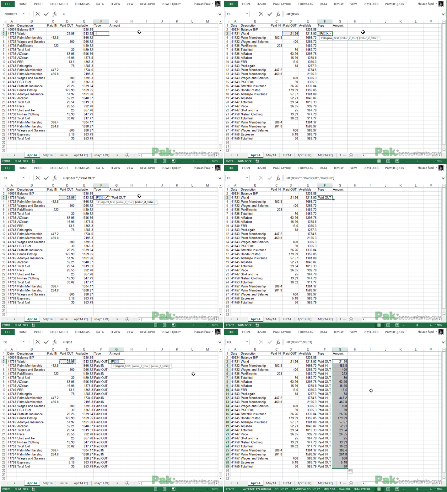
Normalizing data for pivot table manually

Step 1: Go to Apr’14 worksheet and in cell F1 enter “Type” and in cell G1 enter “Amount”

Step 2: In cell F3 enter the following formula and drag the fill handle down to cell F29:

=IF(D3<>””,”Paid Out”,”Paid In”)

Step 3: In cell G3 enter the following formula and drag the fill handle down to cell G29:

=IF(D3<>””,D3,C3)

Now you can delete the columns C, D and E if you want to and even if they stay there they won’t hinder our process. We now only need Date, Description, Type and Amount column for our report.

Repeat the above steps with other two worksheets to have the Type and Amount column.

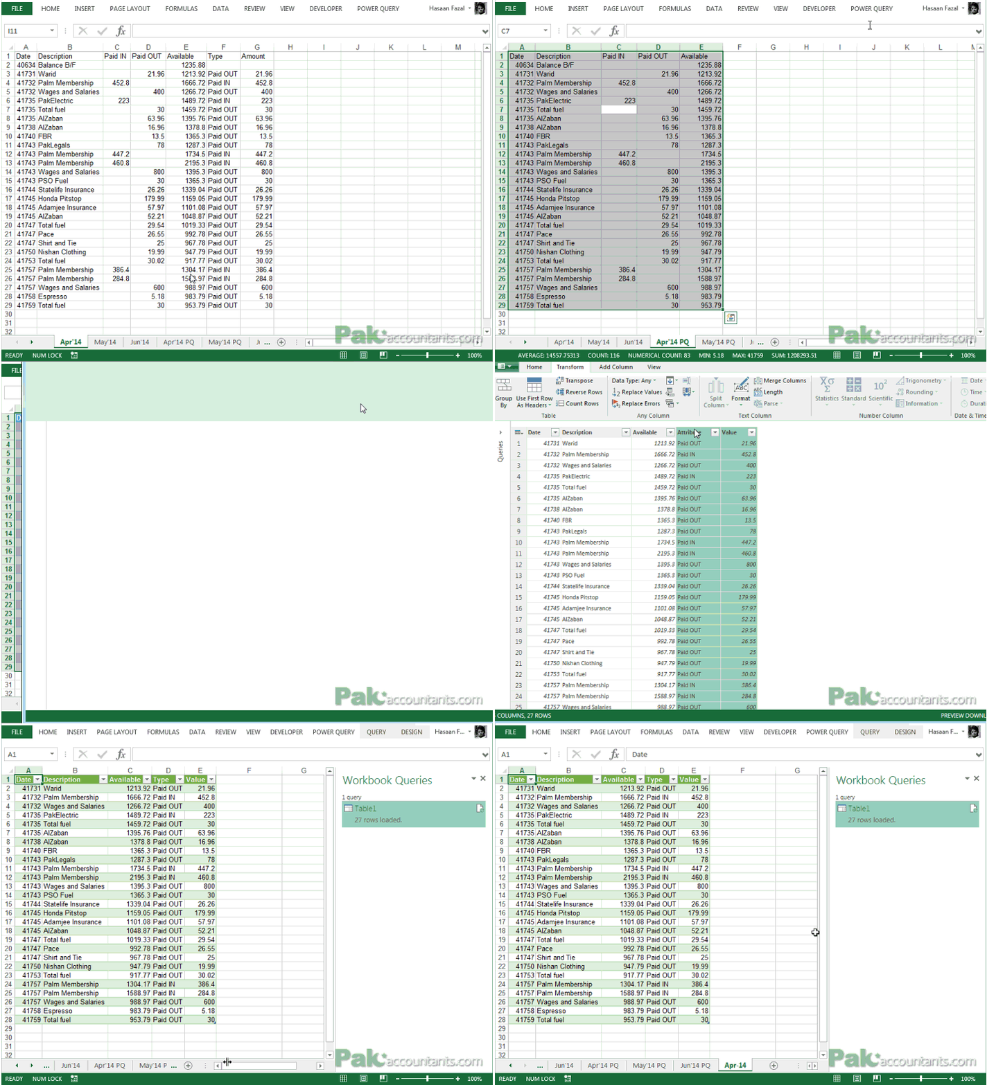
Normalizing data for pivot table using Power Query

With power query we will doing the exact same thing as we did manually but it will save us few minutes. Especially if we have loads of data. Power query will make it super quick and accurate.

Go to worksheet Apr’14 PQ. It has the same data as Apr’14 but just to practice power query its better if we do it on a separate worksheet.

Step 1: Select the whole range, go to Power Query and click “From Table”. Make sure you have “My table has headers” option is ticked and click OK.

Step 2: Select Paid IN and Paid OUT columns by holding down Shift key or Ctrl key.

Step 3: Go to Transform tab > click Unpivot columns.

Step 4: Rename Attribute to Type after double clicking the cell/header.

Step 5: Go to Home tab and click Close and Load button. A normalize table will be inserted in a new worksheet. Rename the worksheet to Apr-14.

Repeat the same steps with other two worksheets namely May’14 PQ and Jun’14 PQ.

Now that we have the normalized data, we have two ways:

1. Either
   use consolidation ranges to let pivot table combine the data. For this I will use Apr’14, May’14 and Jun’14 worksheet’s data.
2. Or
   use Power Query to append/combine the data and then do pivot table on appended data. For this I will use newly added worksheets out of Power Query Apr-14, May-14 and Jun-14.

Cash Flow Summary using Consolidation ranges and Pivot table

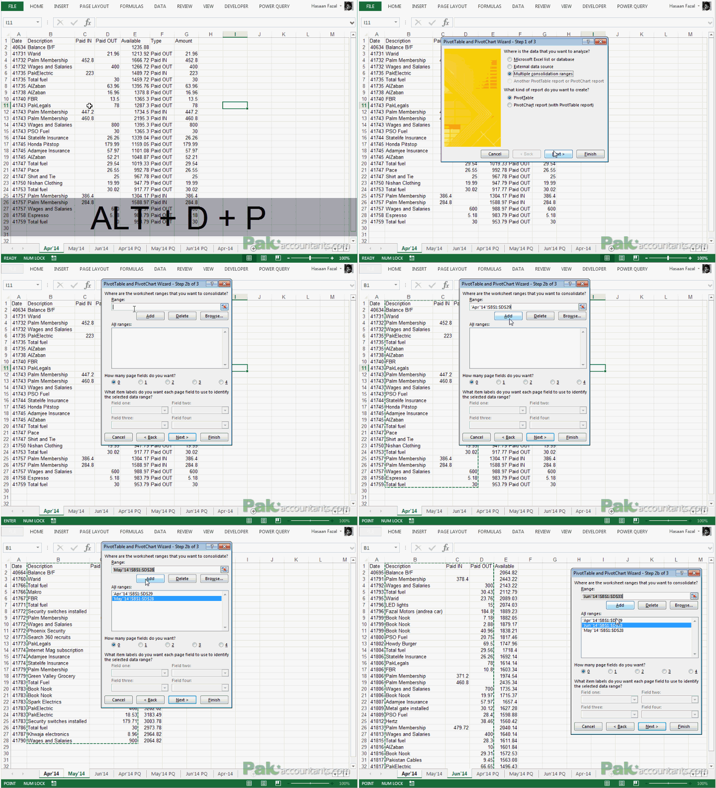
Step 1: Hit shortcut combo ALT+D+P. It will invoke Pivot table wizard. Select multiple consolidation ranges option and click Next button.

Step 2: Select “I will create the page fields” and click next.

Step 3: Start selecting a range from worksheet Apr’14 with columns of Description, Paid-in and Paid-out selected. ONLY these three. Click Add button

Step 4: Repeat the same process with other for worksheets and have them added.

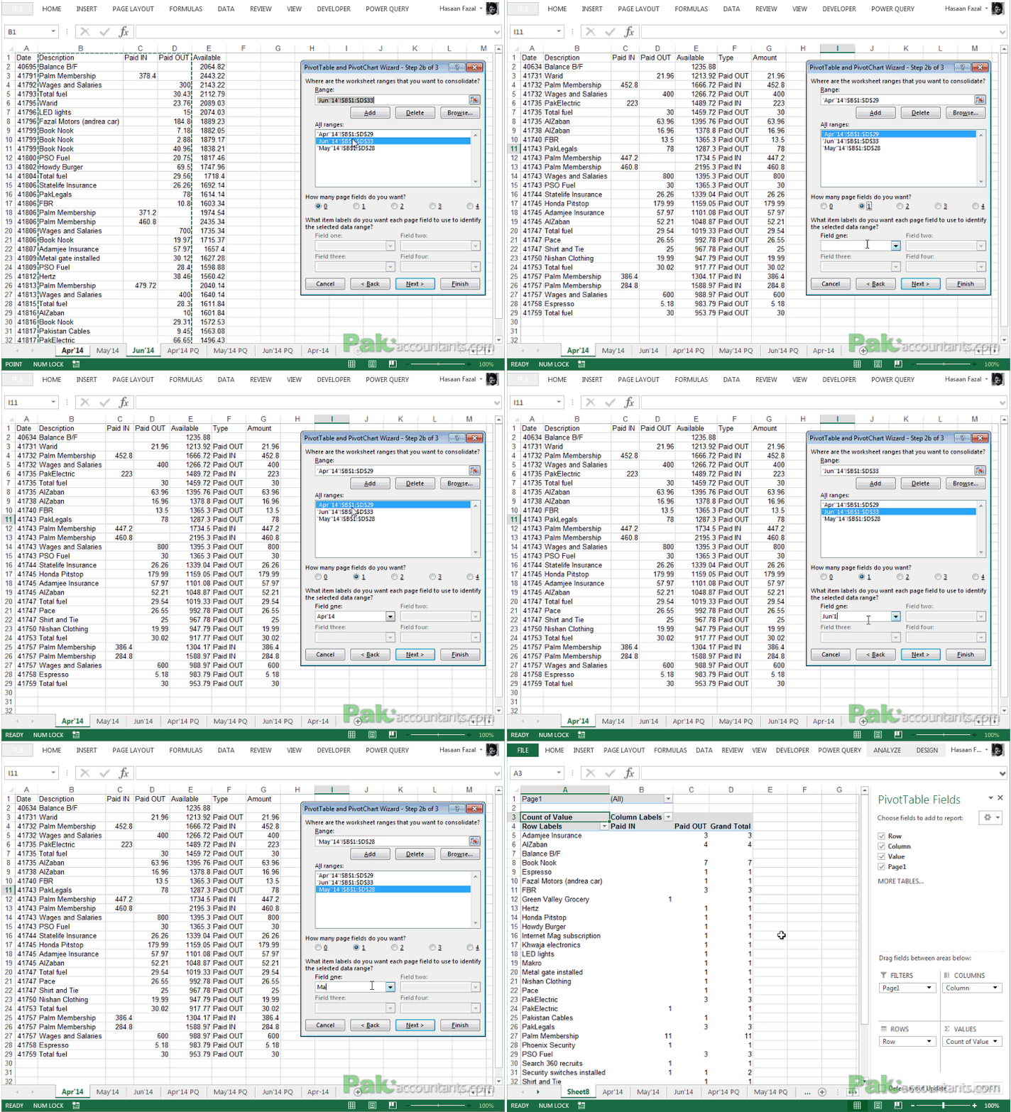
Step 5: Select “1” to mention page fields for each of the range selected. Click the range and give it appropriate name. For the date from April 2014 I mentioned Apr’14 and so on.

Step 6: Once done click Next and then select the option to insert pivot table on new worksheet and click Finish button.

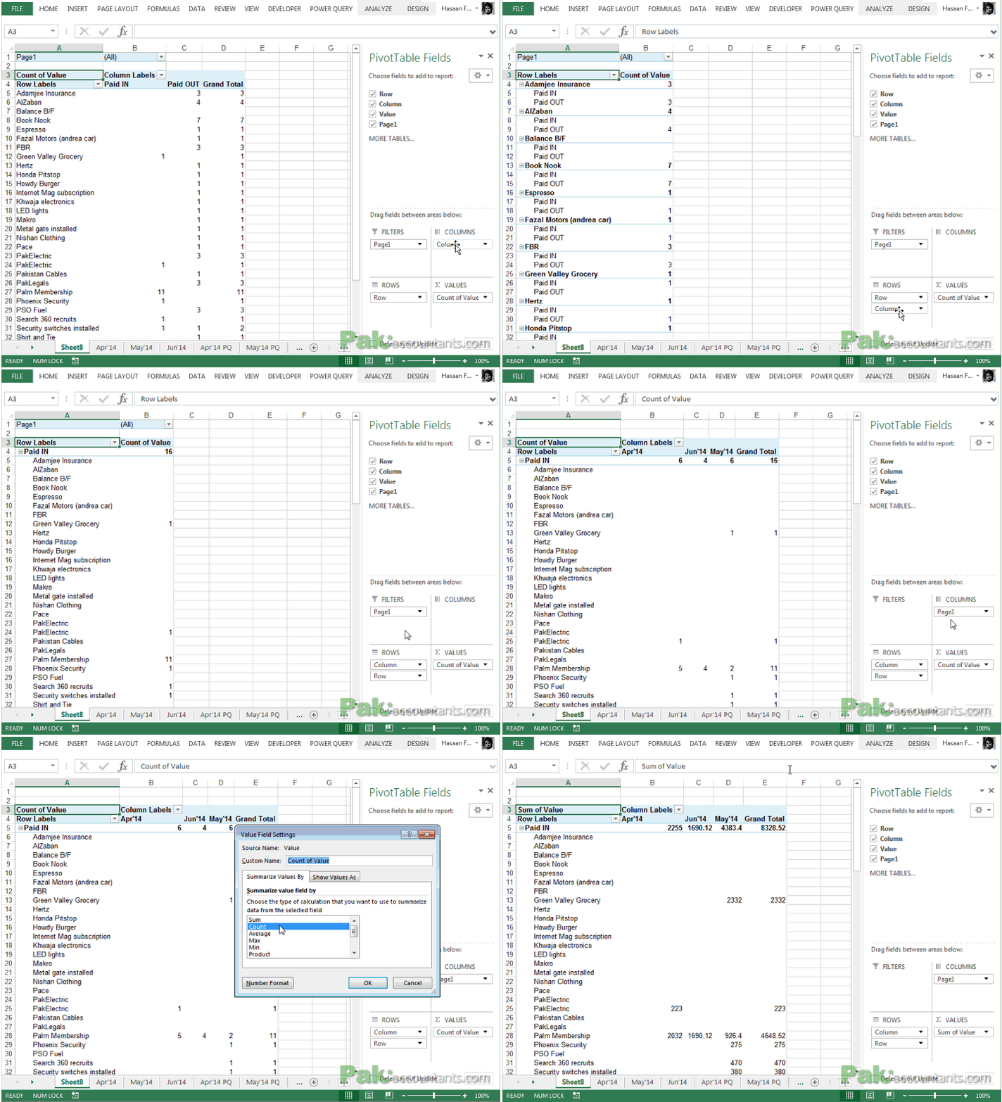
Step 7: Drag the Page field to Columns box, Value field to values box, Column field to row box and drag row field to row box below column field. You might also have to change the way values are summarized. In my case, it was “Sum by count” change it to Sum as shown in the illustration below:

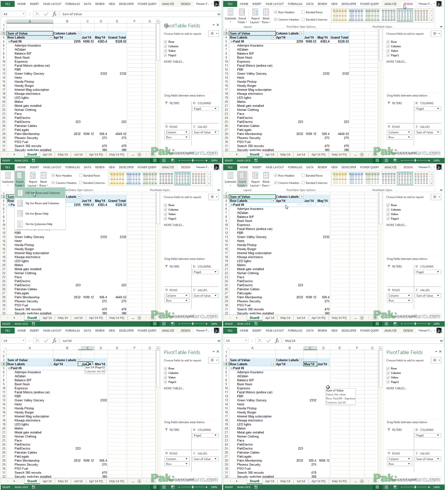
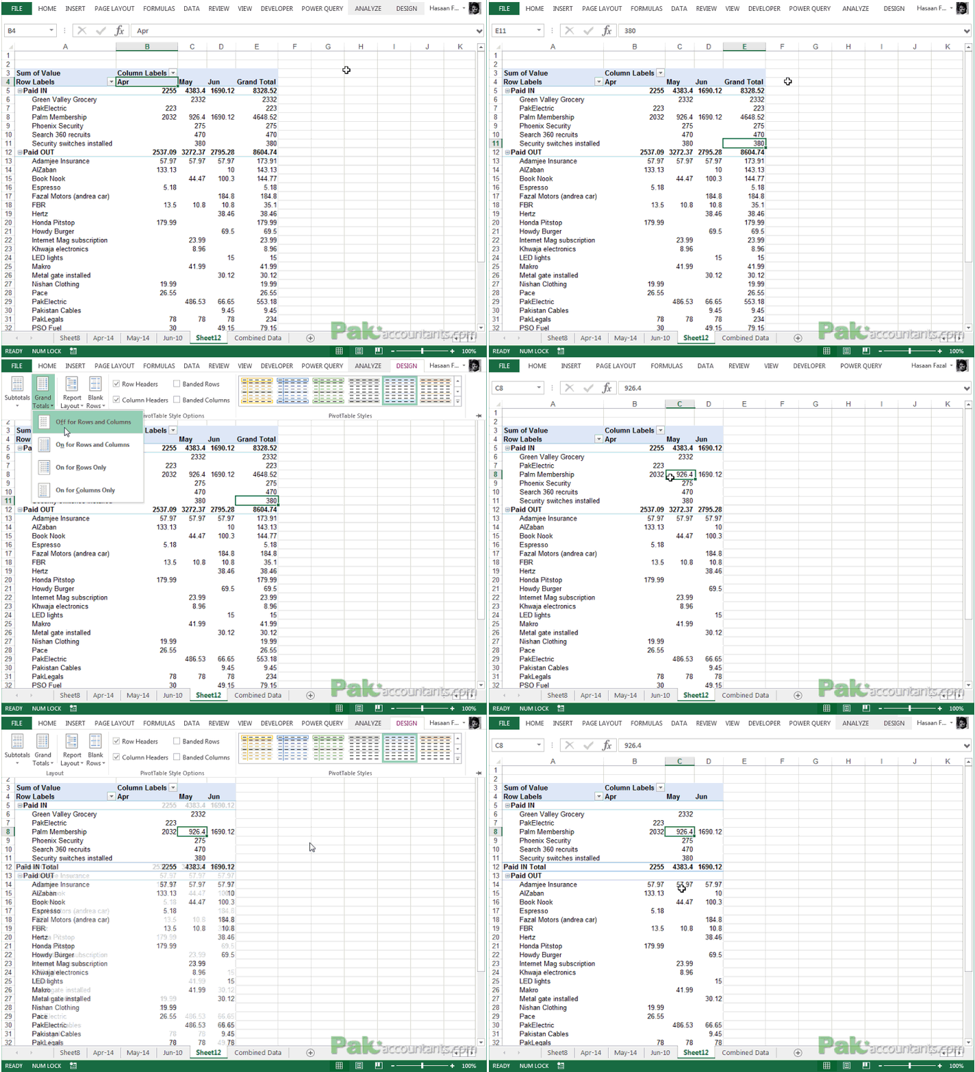
Step 8: You will get a pivot table with report divided in Paid IN section and Paid OUT sections. To clean up the report to make it look as intended turn off the grand totals and make the subtotals appear bottom of the group. Following illustration will help you understand these changes.

You might have to shift a column to make the series appropriate, as I had to move June column to far right.

Step 9: Now to complete the summary we need to add few more lines to our worksheet to make the calculations for closing balance of cash for each period.

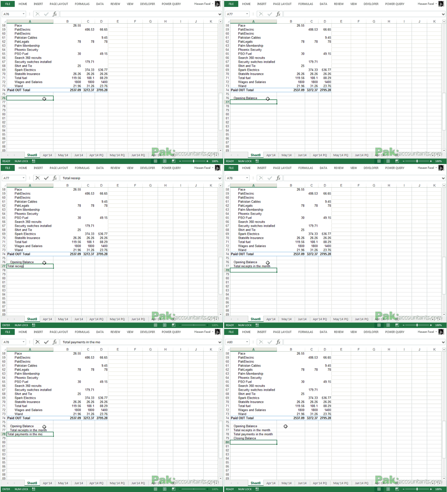
So scroll down and just below the pivot table and make a small format as shown below to make the calculations and summary more meaningful.

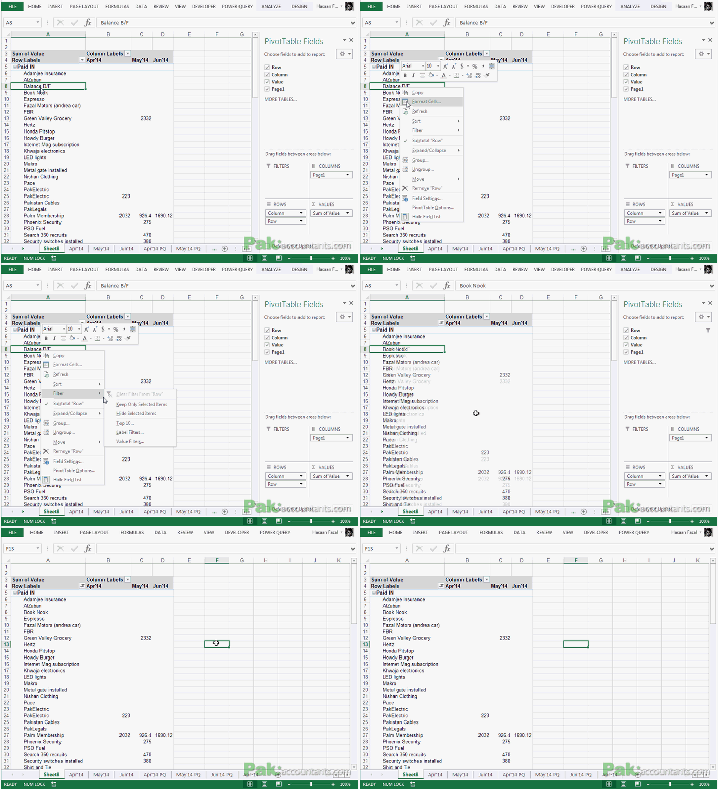
Step 10: One thing I forgot is to hide Balance B/F field from the report. Though its not doing any harm, but its not needed inside Pivot report. So simply right click on it and hide it.

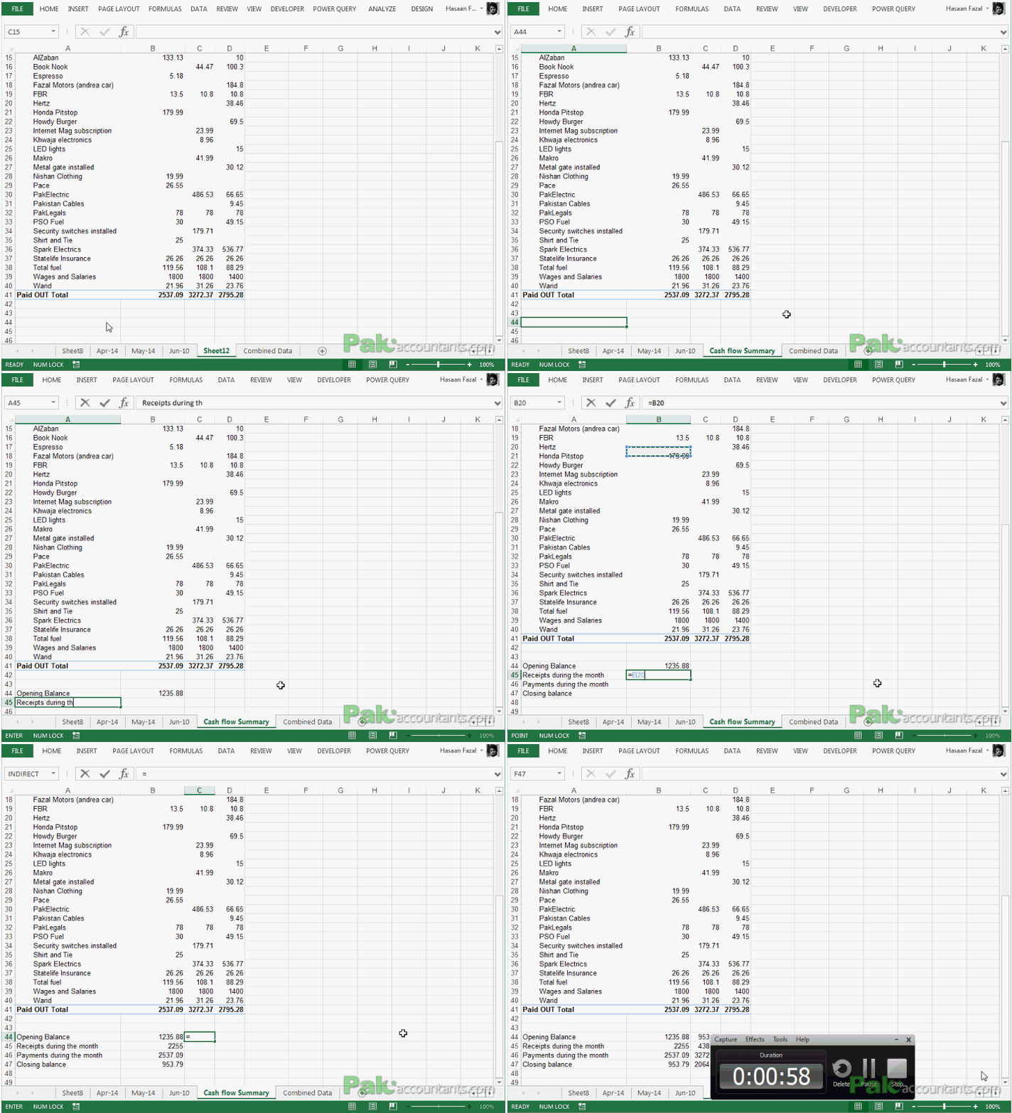
Step 11: Now from Apr’14 worksheet we know the opening balance or Balance B/F was 1235.88 so same will go as opening balance for the month of April in cell B76. In cell B77 we can get the value from the subtotal of total receipts above from the pivot table report. And same way the payments total. Later for closing balance we have to write a simple formula as below:

=B76+B77-B78

The closing balance of April will be opening balance for the month of May so you can give a reference to that cell. Rest simply drag the cells from left and Excel will make the calculations automatically and later dragging the whole data (including opening balance) further to the right to make the calculations even for the month of June.

Consolidation ranges: Why it is not my favourite

Though it does the job, but its crude and the output might not be the one you would like to show to your boss or present in executive meeting. Reason is that Receipts and Payments sections have all the elements whereas receipts should have only those elements that have receipts and payments section should have only those transactions that are payments. This leads to empty rows in both Paid IN and Paid OUT sections:

It is because of consolidation ranges limitations as this feature take all the columns as one entity and thus the flexibility of pivot tables to take each column as separate field is not available. And thus the annoying repetition. I am so far unable to overcome this limitation of consolidation ranges easily. There may be a way using Visual Basic but its unknown to me. But to really overcome you have to make individual reports for each month and then consolidate them. Too much work! For me not practical. If there is a way I would love to know!

So the other way around is to use Power Query to combine the data first and then making the pivot tables. That way our report will not be cluttered and will be formatted properly as it must be.

Cash flow summary using Power Query and Pivot table

First we need to combine the data at one place. If you have already normalized the data using power query method as discussed above then we don’t have to do much. In our case we already have and remember we named those worksheets as Apr-14, May-14 and Jun-14.

If you have not already “unpivot” the columns then for your reference I am putting the steps in the form of illustration again that I applied to “unpivot” Apr’14 PQ worksheet. Simply repeat this process for May’14 PQ and Jun’14 PQ worksheet as well.

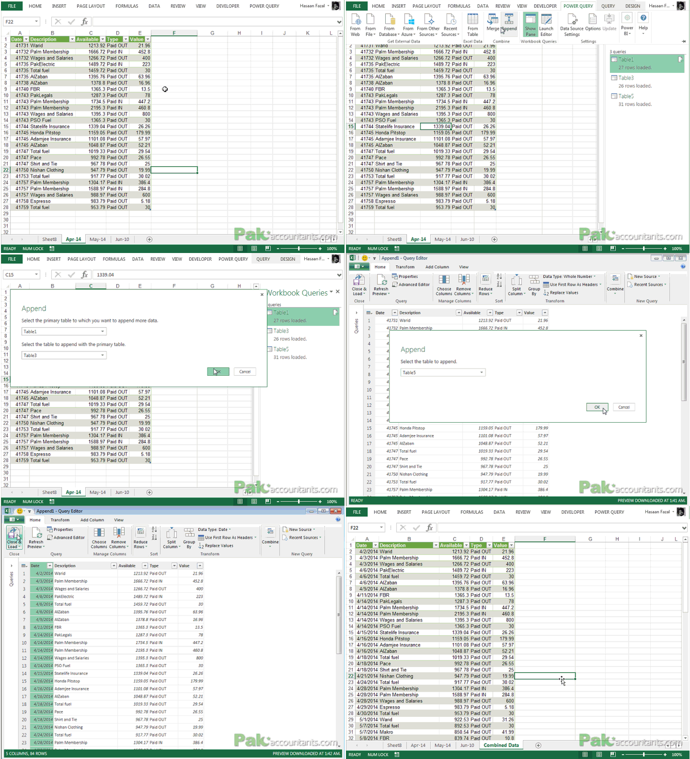
Step 1: Click on worksheet Apr-14 tab and have an active cell within the table. Go to power query tab > click Append button in combine group.

Step 2: From the drop down select the table that relates to April 2014 data and from the drop down below select the table that relates to May 2014. Click OK button. A new window will open with data combined in one column. Click the combine drop down button in the ribbon and click Append query button. From the drop down select the table that relates to June 2014 data and click OK. It will add the data to the table.

Step 3: Right click on Date column header and from the sub-menu go to change type > click Date. It will format the date column correctly.

Step 4: Click Close and Load button under Home tab. It will insert a new worksheet with combined data from all three months. Rename the sheet as you desire.

Step 5: Select the table hitting Ctrl+A and go to Insert tab > click Pivot tables button.

Step 6: Move the fields as follows:

• Date field to column box
• Type field to row box
• Description field to row box after/below type field
• Value field to value box

Step 7: Highlight any cell with date and go to Analyze tab > Click group selection button. From the dialogue box highlight months and click OK button. It will group the dates in months.

Step 8: To clean up the report go to design tab, turn off grand totals and show subtotals under each group.

As you can see it is way better than the report we generated using consolidation ranges discussed above. It is much more understandable, formal and ready to be used anywhere.

Just like we did earlier, we have to make opening and closing balance calculations. Now its as easy as eating cake! Following animation shows the final calculations made make the summary complete with opening and closing cash balance calculations.

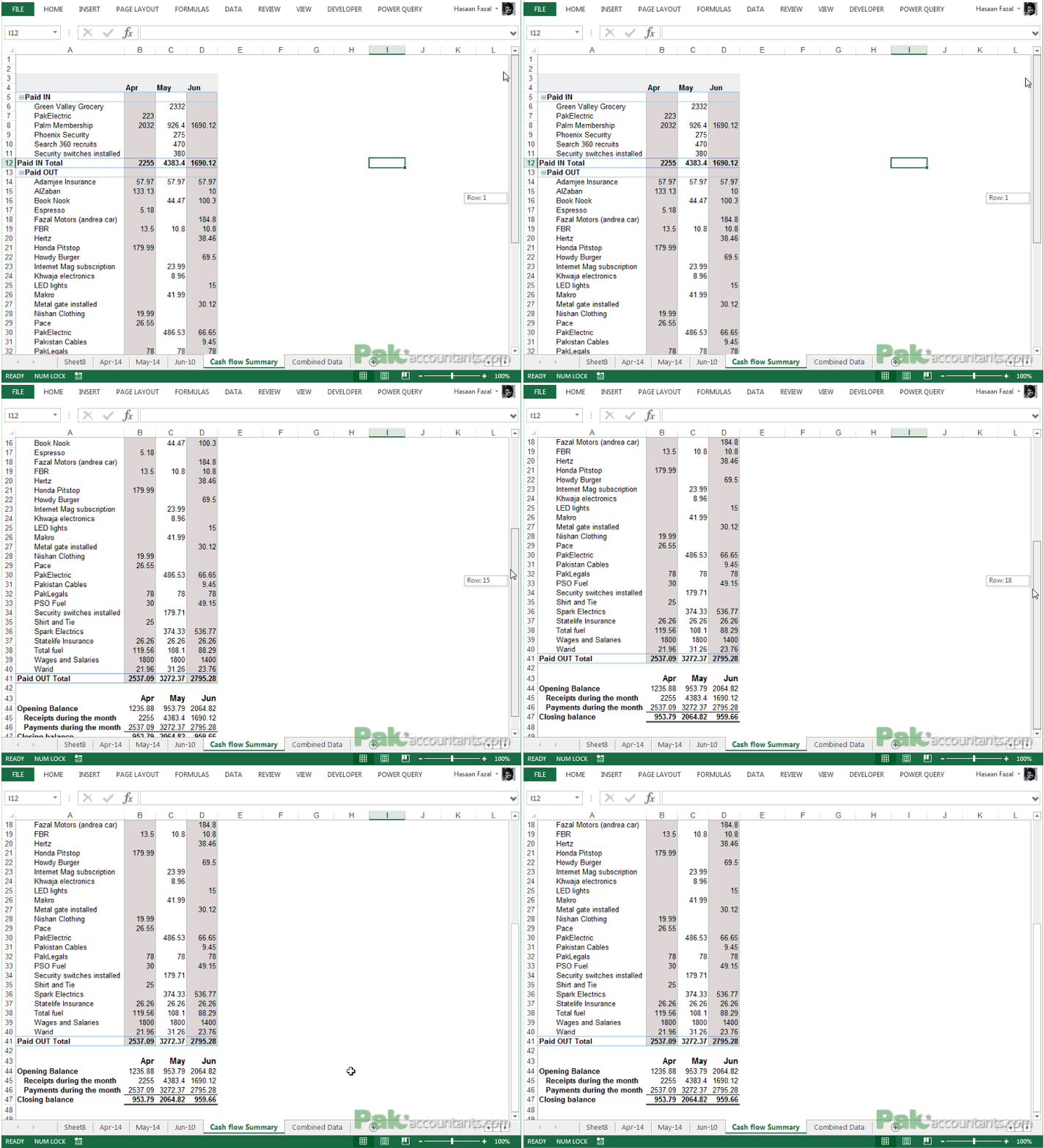
With a little more changes and formatting tweaks this is what I ended up with:

Right! This was lengthy! I admit! But it was so much FUN! And I hope you must have enjoyed this detailed tutorial as much I did writing and working on it.