How to show data of hidden rows/columns in Excel Charts

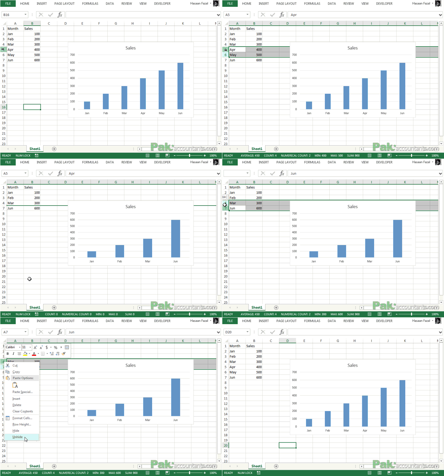
 By default if you hide a certain row or column of a data on which a chart is based, Excel will automatically hide that data too. I must confess that I was quite annoyed when I wasn’t able to have a control over this behaviour as sometimes I do need to hide the data but still want data in the chart.

But its easy to handle. To show the hidden data or data of hidden cells, rows or columns simply do this:

Have your chart active > Go to design tab > Click select data button in data group > A dialogue box will open > click Hidden and Empty cells > A dialogue box will pop up > check mark Show the data in hidden rows and columns > Click OK.

Now even if you hide the data, chart will still show the data plotted as normal.

See! Told ya its easy!