How to LOOKUP using ONLY Conditional Formatting in Excel

 Few days back we learnt how to do 2-way lookup i.e. looking up the value against two criteria. You can learn it in detail here: How to do 2 Way Lookup in Excel – One value to lookup with two criteria using Intersect Operator

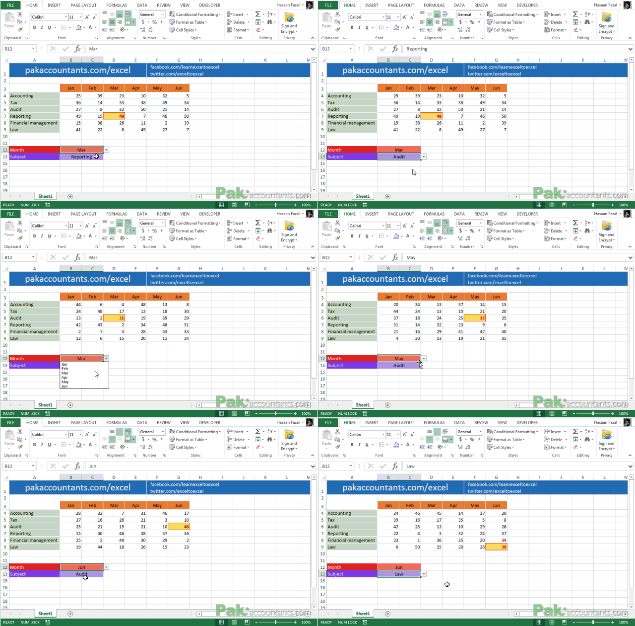
In the tutorial mentioned before the value was fetched in a separate cell outside the original data. Though it is practical and can be used further but what if we just want to highlight the value? Following animation shows what we are after:

The beauty of this technique is that it is extremely simple yet effective. But this is only good if you want to see the value and not actually going to use it for subsequent calculations.

Download Tutorial Workbook

Download this excel workbook that provides you with basic data to apply the steps discussed in this tutorial

LOOKUP using Conditional Formatting

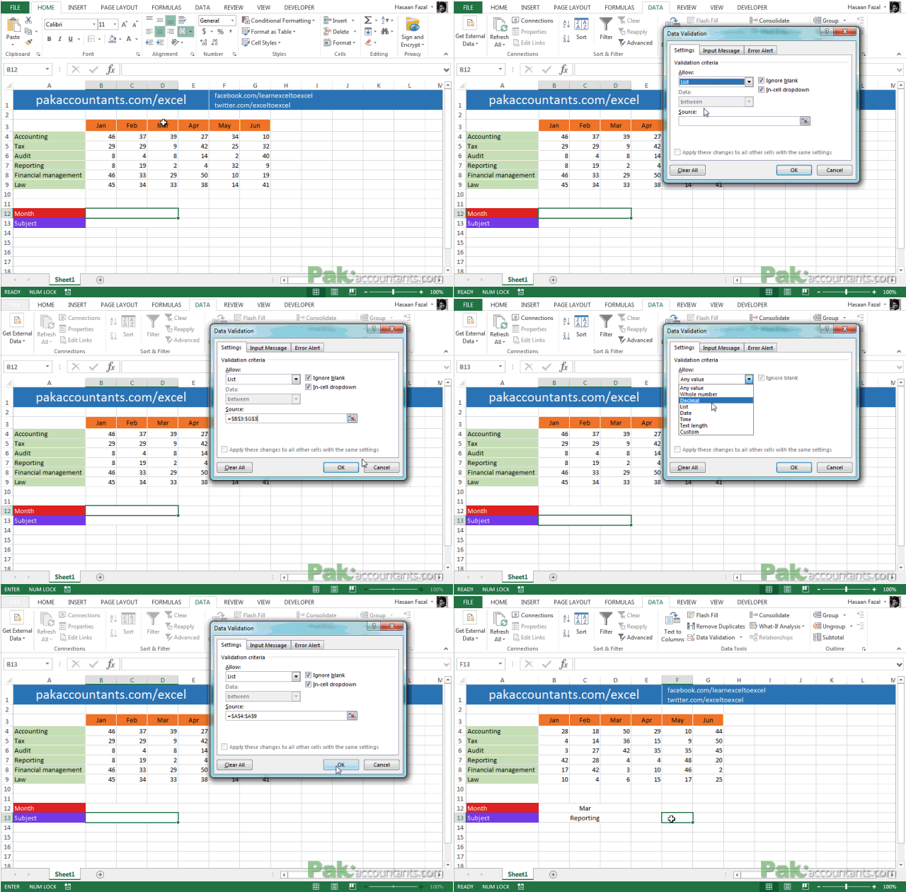
Step 0: Just to make it work smoothly, its better to have drop down lists using data validation tools. We need drop down lists for both Months and Subjects. Following animation will walk you through how to get it done:

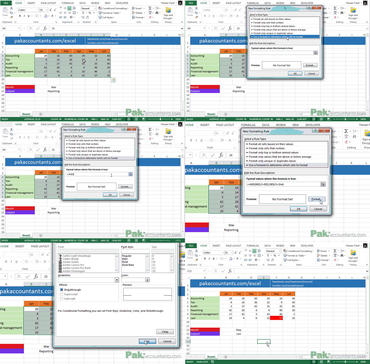
Step 1: Select the data excluding the column and row headers.

Step 2: Go to Home tab > Styles group > click conditional formatting drop down > Click new rule.

Step 3: Select the last option i.e. use a formula to determine which cells to format

Step 4: Put this formula in the input bar:

=AND($B$12=B$3,$B$13=$A4)

Step 5: Click the format button and select the color and adjust font or add borders the way you desire so that lookup value is easily identifiable. I selected red color with white font color to make the lookup value stand out. Click OK.

Following animated illustration will walk you through all the five steps:

AND done! Yes! Thats it! Snappy isn’t it 🙂

Now if you change the Month or Subject then corresponding number of lectures will be highlighted.

Understanding the formula

The formula in step 4 is checking for two logical tests:

1. first: if $B$12=B$3
2. second: if $B$13=$A4

If both conditions are true then the resultant will be TRUE and thus a cell will be formatted with the selected changes made in Step 5. Remember B12 is the cell in which we select the month and B13 is the cell in which we select the subject

But the question still remains how the cells are getting highlighted as we are only checking about subjects and months?

Well the reason they are highlighted is that conditional formatting feature will format the cell with selected colors and font style if the formula returns TRUE value. Now we are carrying out these logical tests in all the cells at the same time. For only one cell the result will be TRUE and for the rest FALSE and thus only one cell will be colored or highlighted.