Grand Totals to the left of Excel Pivot Table instead of default right
In pivot tables by default grand totals appear at the right end of the report. But sometimes the pivot table is so wide that user just can’t see the grand totals and we have to scroll every time we need to refer to that cell.
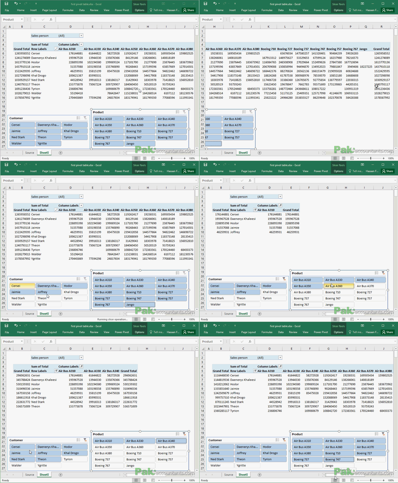
Situation is even more frustrating if the width of pivot table is changing. For example in if you have slicers in place and every time report is filtered the width changes.
In short, the right end is not all the time visible and is also shifting places. And it is happening just because it is at the RIGHT of pivot table. Problem will be solved if somehow we can have grand totals to the LEFT of the pivot table!
If we have the grand totals at the left, it will not only be visible all the time but also won’t be shifting places every time we filter the report. It would be awesome if Excel provided us with such option right inside pivot table layout options but its not! So we have to improvise and yes there is a workaround and once applied following is the result!
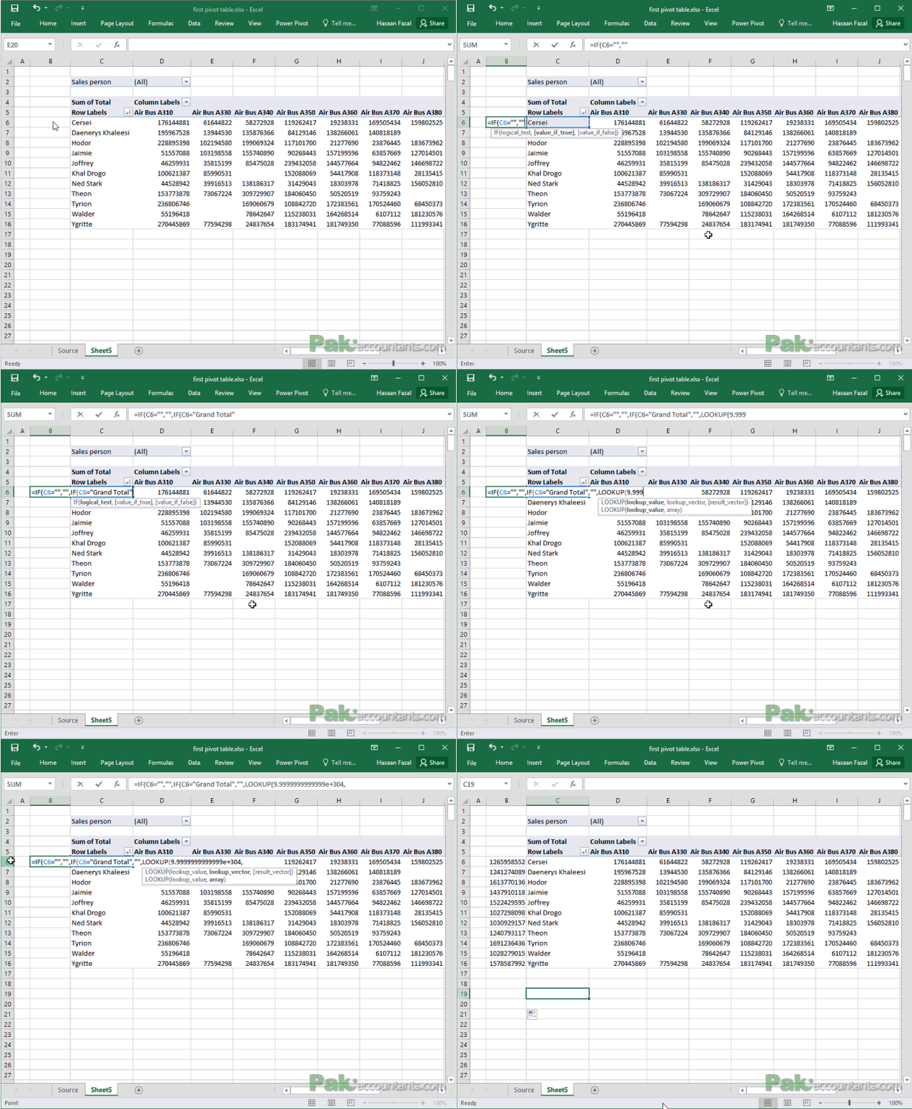
To get the grand totals column at the left, insert a new column at left if you don’t already have the space for it. Then put the following formula in the cell adjacent to the first cell of pivot table containing records:
=IF(C6=””,””,IF(C6=”Grand Total”,””,LOOKUP(9.99999999999999E+304,6:6)))
Drag the fill handle down as far as appropriate so that calculations are visible even if pivot table attains maximum length down the columns.
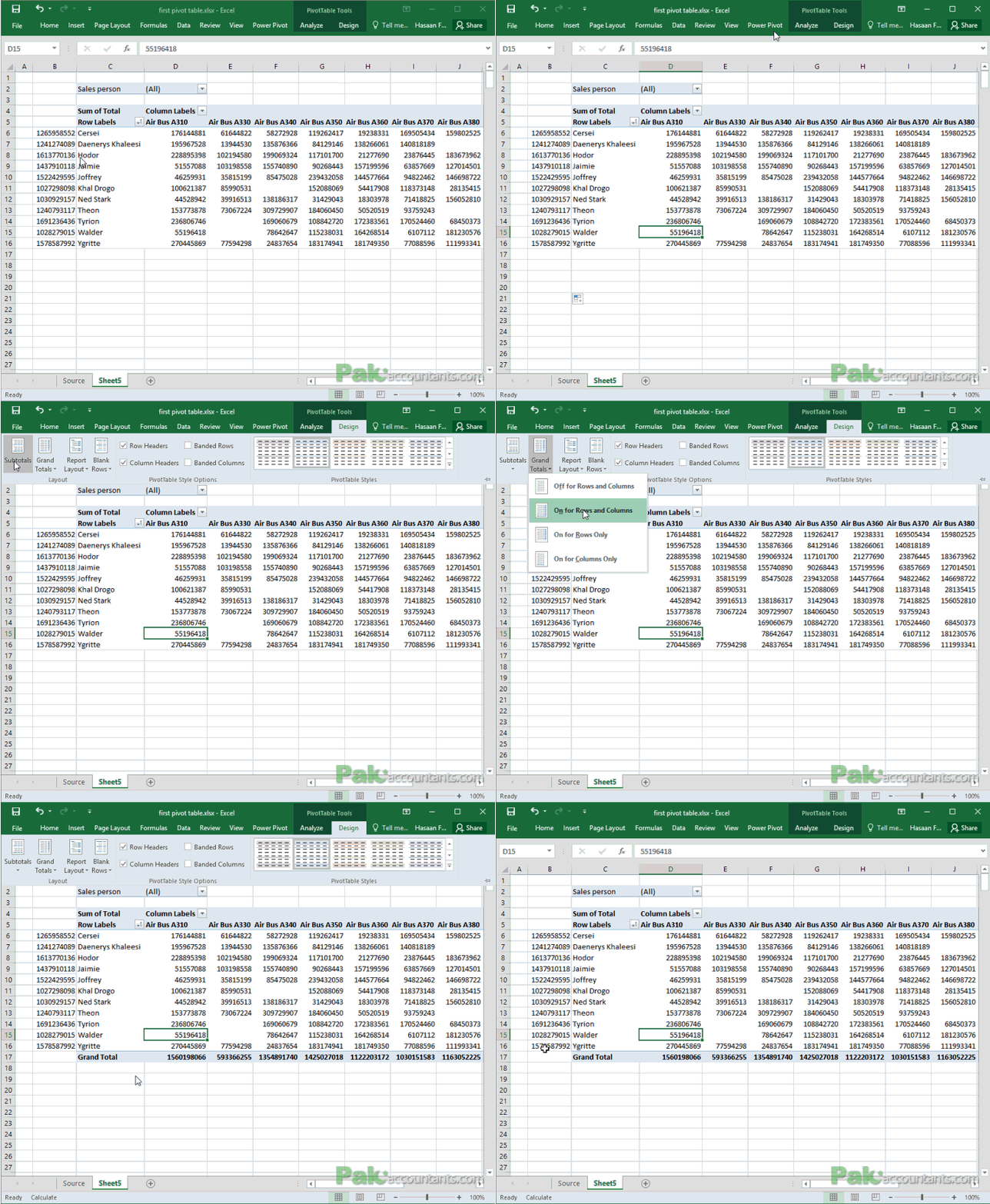
One last thing to mention is the reason of using two IF() functions. I wanted grand totals of individual records only and not the total of grand totals. And even if the grand total option is enabled, it won’t show up as it can be seen in the following illustration:
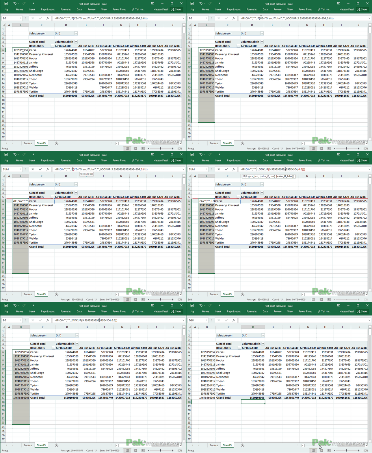
But if you like to have it then modify the formula slightly in which case the formula will become:
=IF(C6=””,””,LOOKUP(9.9999999999999E+304,6:6))
And now you can see that even grand total figure is visible:
Now with few formatting tweaks like coloring few cells, giving heading and disable grid view under page layout tab, its show time with slicers enabled!


Leave a Comment