Extract First and Last word from text string using Excel Formula

Extract First and Last word from text string using Excel Formula

Say you have several text strings and you want to separate the first and last words from each text string using Excel. This can easily be done using Excel formulas and a going little clever with them.

Extracting first word from text string

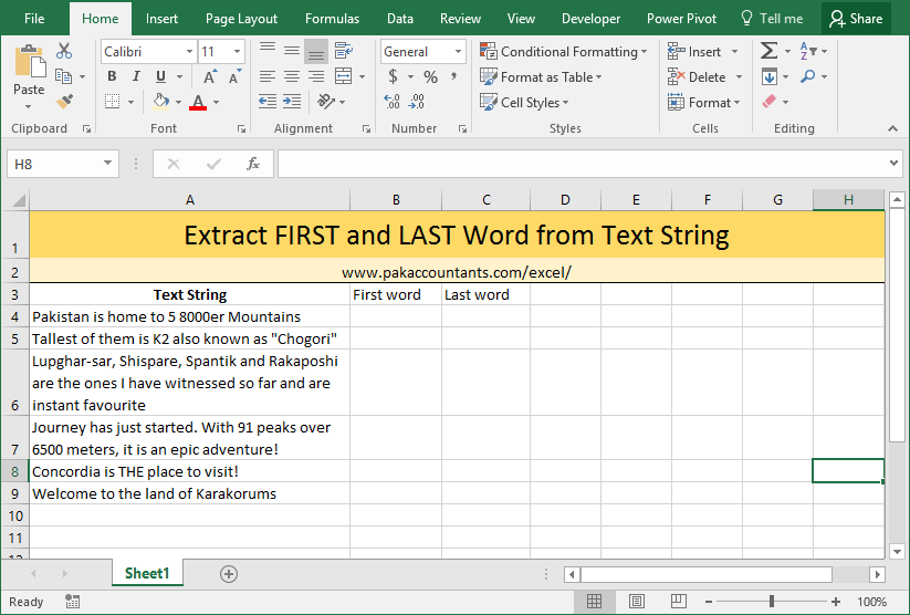
Consider the following set of strings in column A:

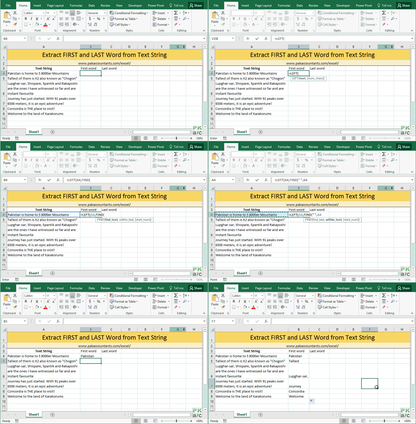
To extract the FIRST word I used the following formula in cell B4:

=LEFT(A4,FIND(" ",A4)-1)

Double click the fill handle to populate the whole range.

Fairly simple formula. Starting from the inside, FIND function is finds the location of first “space” in cell A4. FIND function will return a number which is simple telling the location of “space” in Nth character form. In first case for example it is 9 as space is the ninth character starting from left. Pakistan is 8 character long.

Now that we know that first space is at 9th place, it means first word is 8 characters long, therefore using LEFT function and asking to extract 9-1 characters from the cell starting from left will yield us first word in the text string.

Extracting LAST word from text string

Now this is a little tricky one. Tricky because Excel’s FIND function has limitation i.e. it can start looking only from left to right and NOT from right to left. I really think it is possible as Microsoft only has to insert an optional argument as TRUE, FALSE to change the direction of lookup. But no help so far!

So we have to go for workarounds.

Again presenting the situation:

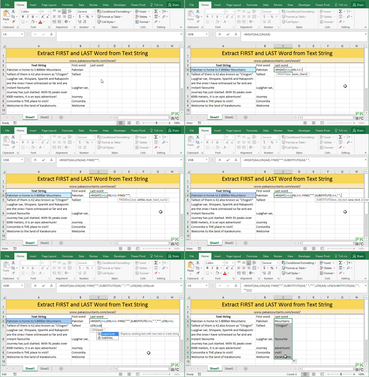
To get the last word from text string I used the following formula:

=RIGHT(A4,LEN(A4)-FIND("~",SUBSTITUTE(A4," ","~",LEN(A4)-LEN(SUBSTITUTE(A4," ","")))))

Yeah its a pretty sandwich of RIGHT, LEN, FIND and SUBSTITUTE functions that does the job! Just double click the fill handle to populate down the range.

So what is happening in this formula. Let me break it down for you so that you can understand it better:

1	=RIGHT(A4,
2		LEN(A4)-
3			FIND(“~”,
4				SUBSTITUTE(A4,” “,”~”,
5					LEN(A4)-
6						LEN(SUBSTITUTE(A4,” “,””)
7							))))

Right!

So we have the formula in steps that I think will be easy for me to make you understand.

Line 6:

Starting from line 6; what we have is SUBSTITUTE swallowed by LEN. SUBSTITUTE function is basically substituting any “space” for “nothing” i.e. SUBSTITUTE function is removing spaces from the text string mentioned in cell A4. Once removed it will give to LEN function which will tell the number of characters in the result just given by cell SUBSTITUTE.

Didn’t get it? F9! Oh I meant fine!

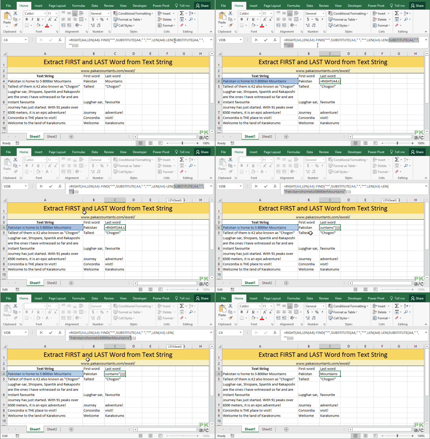
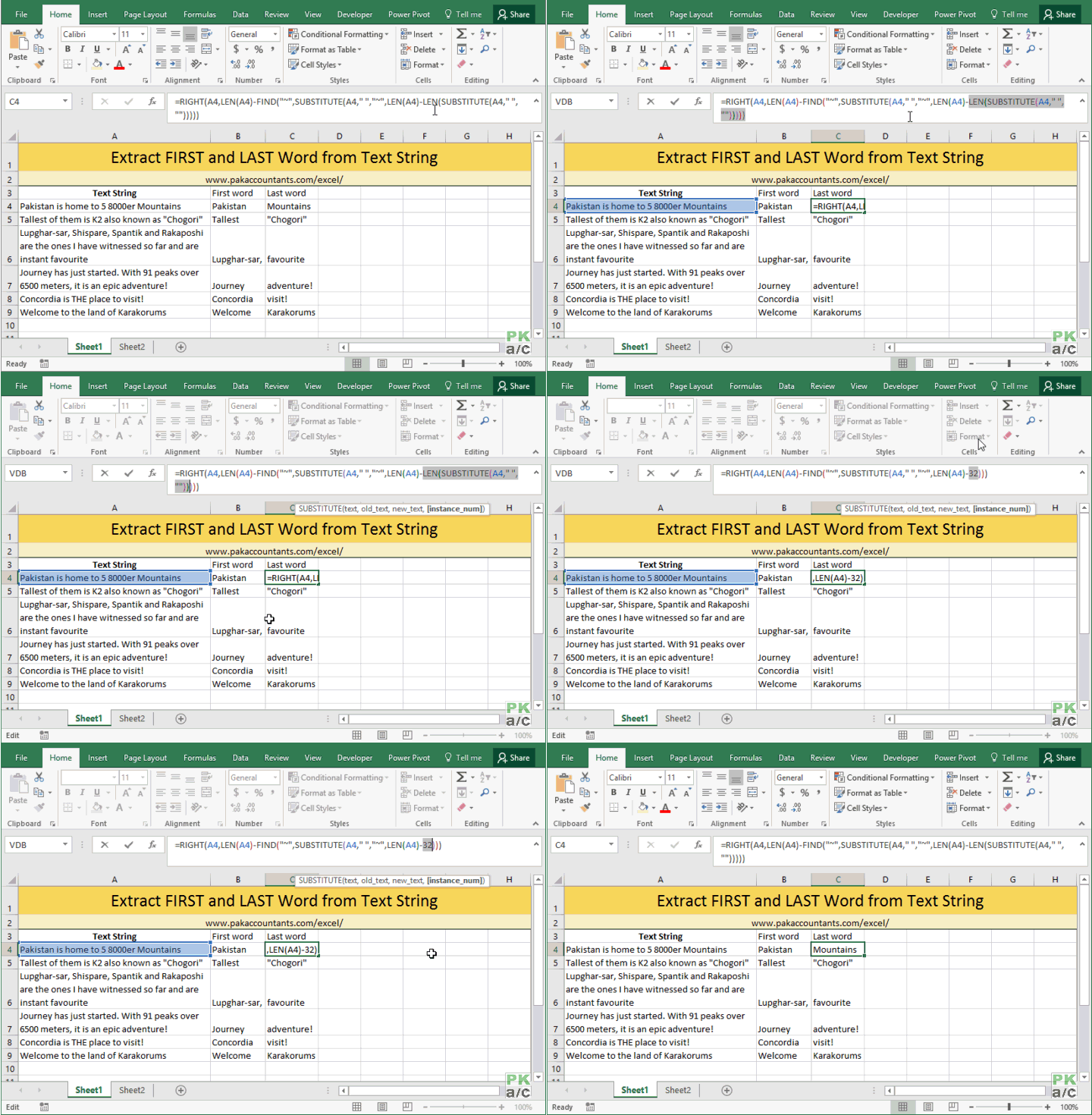
If you select the SUBSTITUTE function and its contents just right and hit F9 key on the keyboard it will give you the results! Press Esc key to discard the changes.

Right so once we have spaces eliminated LEN function will calculate the characters for us that are exactly 32.

So for line 6 we have a result that is 32!

Line 5:

Now moving up to line 5 where we have LEN(A4)- the results from line 6.

Now LEN(A4) will count the characters WITH spaces and will give the count of 38.

So 38-32 gives us 6 which will be fed to line 4 above.

Line 4:

In line 4 we have SUBSTITUTE function again and this time its substituting space with tilde “~” BUT only a specific instance. Remember the syntax of SUBSTITUTE function is:

=SUBSTITUTE(text,old_text,new_text,[instance_num])

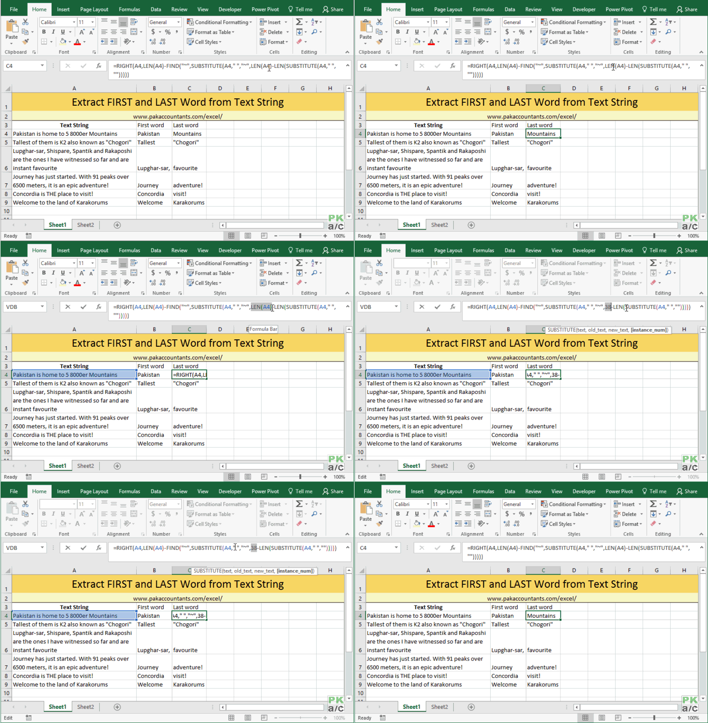
[instance_num] is an optional argument which if used tells Excel to substitute ONLY this instance and not all. We obtained the value for this instance from the results of line 5 and 6 which is 4!

Now 4th space is the last space in the text string. For which we are substitute a character “~”.

The result if you try to preview with F9 in formula bar is as following:

Line 3:

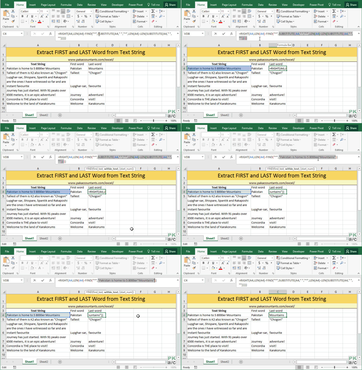
Now that we have substituted the last space in the text string with a special character we can perform FIND function to look for its location within the string produced as a result of line 4,5 and 6. And this is exactly line 3 is doing find “~”.

This will give us a number again which is 29. This will be given to Line 2 above

(Skipping the F9 animation for this time)

Line 2:

In line 2 again we are counting the characters in A4 with spaces using LEN(A4). Just normal counting which gives us 38. However, the results from line 3 below are subtracted from 38 that leaves us with 9 (38-29). This will then be fed to line 1 above.

Line 1:

In line 1 we have RIGHT function which is trying to extract specific number of characters from a text string mentioned in cell A4 starting from right.

Now this specific number is a result of line 2 which is 9. Therefore, RIGHT function will extract NINE characters from the text string in cell A4 from the right. And those 9 characters in current situation are Mountains which is basically the last word of the text string.

COOL RIGHT! I hope the above demystification process to find the last word had made clear sense to aspiring Excel heads who are just starting on these formulas.

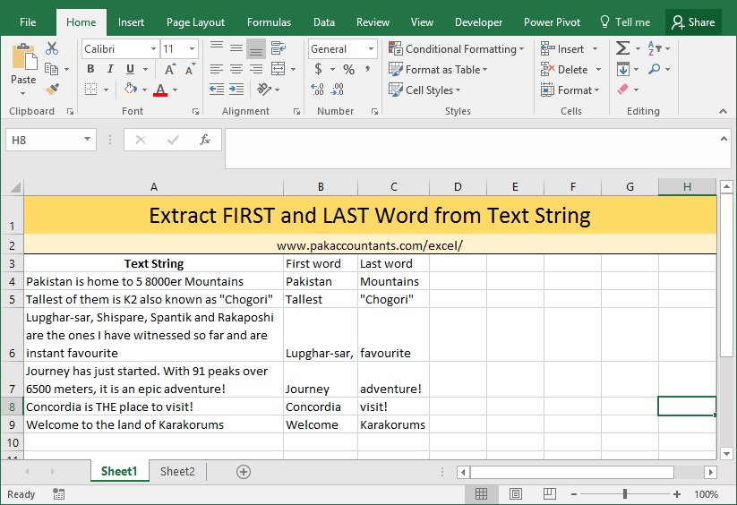
So here is the final result:

What’s Next!

The best way to learn and be better is to keep challenging yourself.

In the final output above you can see that few results are with exclamation marks and quotes. Now if we only want the text and no alpha-numeric characters then how to do it?

I am pretty sure that its all possible in the realm of VBA but I am more interested in formula only approach! Do share your technique in the comments.