Excel Mouse Mayhem – 35+ Mouse tricks for mouse monges

Excel Mouse Mayhem – 35+ Mouse tricks for mouse monges

I know many of the Excel users prefer keyboard shortcuts and Excel does provide plenty of them. But if we are keen to know and remember keyboard tricks then we should pay some homage to PC’s mouse. Following are the double click tricks you can do with your mouse in Excel to make your daily work much more fun.

As always the collection is long and so has been divided in several pages so don’t forget to check other pages to get all of the mouse tricks that you can use in Excel to expedite your daily routine.

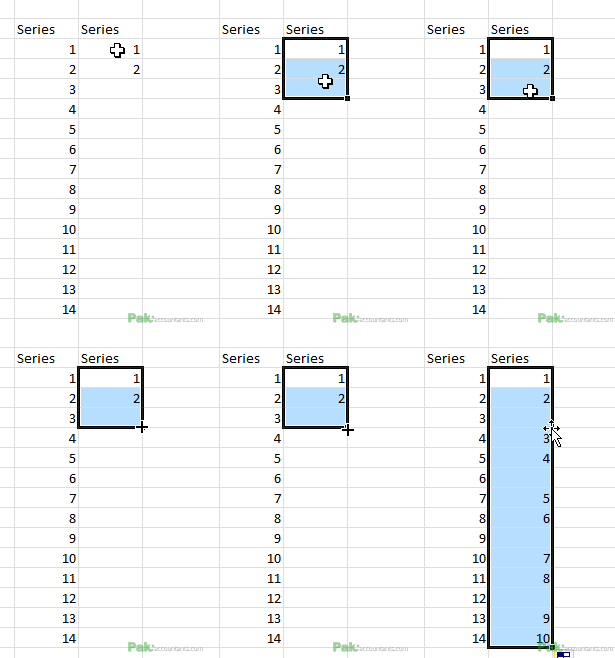
1. Double click fill handle to fill down to whole range – 6 Tricks in 1

This is probably the best double click trick of Excel. If you don’t know it yet then its a must learn trick. Suppose you have a large data set and in one column you have entered the formula. Now you want the same formula in every row down the whole column until the end of range. Normally you would select the whole range and paste the formula. Or drag the fill handle.

Instead of dragging it, just when the mouse turns black + double click the fill handle and ZOOM! the formula or whatever the content of the cell is will be copied down to the last cell of the range. How quick is that. You can do this after inserting the formula in cell

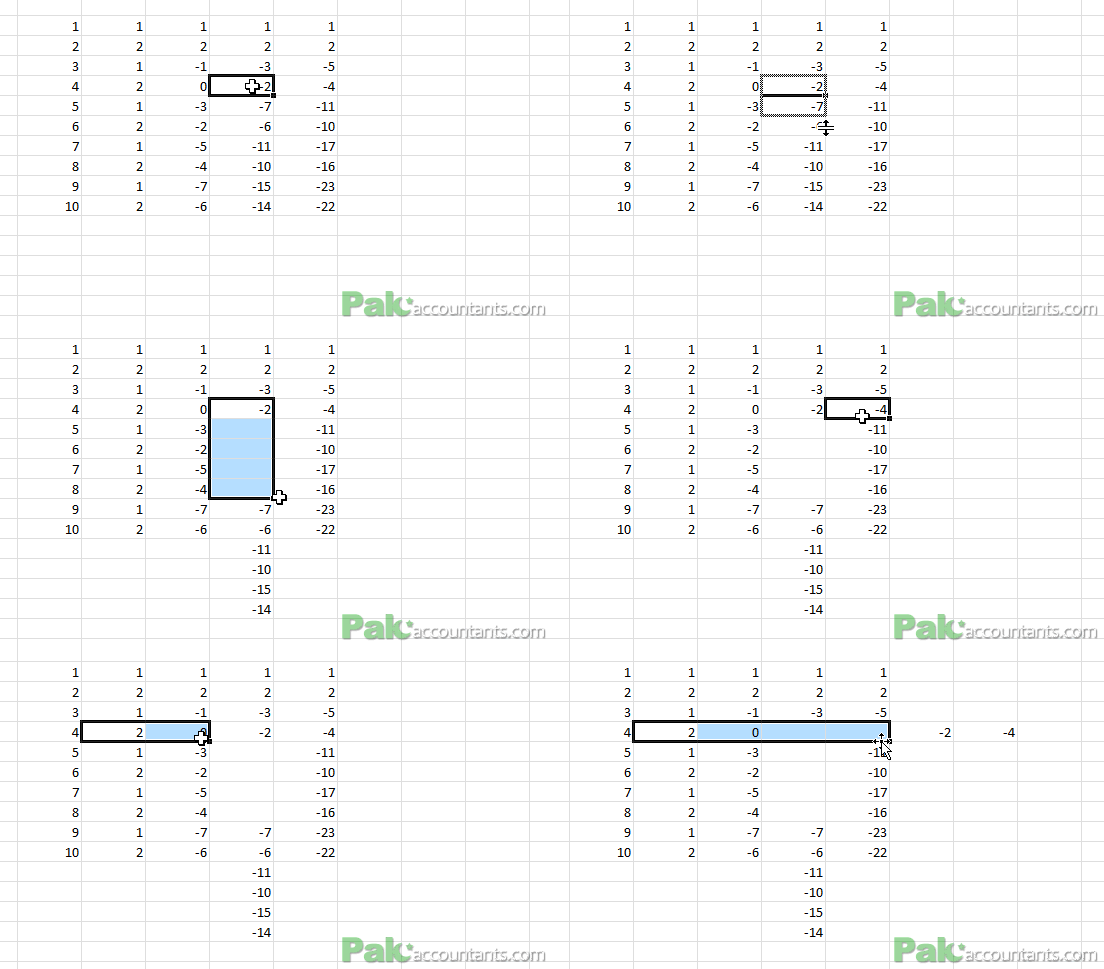
Bonus Tip – Double click fill skipping row(s)

For example you want to insert the content or series or formula skipping equal number of rows for example after every second row, or alternative rows etc. Then select the cell which you want to copy including the number of rows you want to skip and double click fill handle. How awesome is that? 🙂

Known Issues

The behaviour of double click and the way Excel determines the last row of the range is different from version to version. But 2010 is a little better as it use a different approach to identify active range. However, in case of 2007, it checks the adjacent cells and it would continue copying until the last actual cell of range if any cell at left and also on the right is blank. So in 2007 or earlier version you might have to double click several time to completely fill the down to last cell of range.

Bonus Tip – Right click hold and drag

I really wish it could work by double clicking right mouse button but you have to hold and drag. Once you release right click a menu will open from which you can select how you want to fill cells.

Bonus Tip – Hold Ctrl key and drag to copy cells

Sometimes when you drag fill handle excel automatically insert series. Although on releasing the left click you can select copy cells from the smart tag. But if you hold Ctrl key down and then drag (you will notice small plus sign just on the right of cursor) and then drag it, it will copy cells.

Bonus Tip – Drag fill in reverse direction within selection

We already learnt that if we drag the fill handle on empty cells then cell gets filled. However, if you go backwards then cell content gets deleted. Remember that reverse movement must be made after selection otherwise active cell gets copied.

Bonus tip – Hold Shift key to insert rows / columns

If you press and hold Shift key and then drag the fill handle in left or right direction it adds columns in the same row

If you press and hold Shift key and then drag the fill handle in up or down direction it adds rows within same column

2. Double click row / column margin to adjust height and width

Have a long text in cell not appearing properly? Like there is width is too narrow or too big? You can adjust that easily double clicking the column or row splitter or margin. If you want to adjust a column you have to double click the border at its right not the left one. Similarly if you want to adjust the height of specific row you have to double click the bottom splitter and it will expand or contract to appropriately accommodate the content inside it.

You can adjust the width or height of multiple columns and rows in one go using the same technique. Simply select the rows or columns you want to adjust and double click splitter of any row/column inside that selection and all the columns/rows will be adjusted instantly.

3. Double click format painter

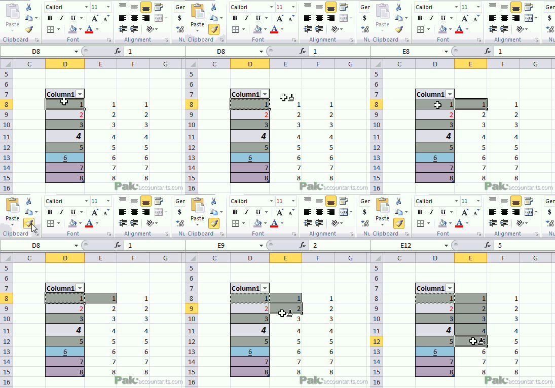
Format painter let you copy the format of specific cell in other cells easily. But if you have several cells to format using this tool then you might be thinking that you have to click format cell button every time. No!

Save yourself time and effort by double clicking the format painter button once and then click on cells you want to paint. Once done hit escape key or click format painter button again in the ribbon to disengage format painter.

Bonus tip – Multiple rows and columns with multiple formats

Format painter is not a simple format paster. It has a good memory of remembering formats of multiple rows and columns that might come with multiple formats and saves you tons of time not repeating those steps again for each cell.

4. Double click formula bar to expand quickly

If you have a long text or a formula in a cell then sometimes even a formula bar cannot accommodate the whole thing. However, if you click the formula bar expandor button then formula bar will expand just enough to show the whole thing. You can do this by double clicking the bottom border of formula bar and it will expand.

5. Double click and hold to select cell content

While in edit mode if you have to select a sentence or argument with in range we usual press and Hold Shift key and drag the mouse with left mouse button pressed down. However, if you double click and hold left mouse button and drag to make the selection. This will free up your hand and you don’t have to keep holding Shift key pressed.

6. Double click pivot table item to drill down

In a pivot table figures are reported on summarized basis usually summed up in one group. If you are interested in knowing that how pivot table calculated this amount then simply double click it and a sub-report or mini report in a new worksheet will be generated detailing how the figure has been reached and reported in pivot table.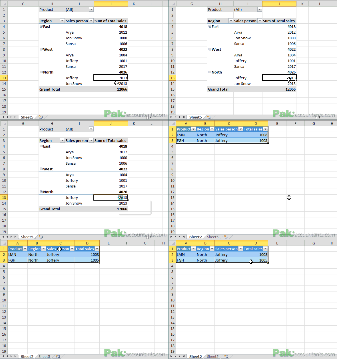

7. Double click splitter to activate split screen

Split screen function let you divide the same worksheet in two or four work zones so that you can easily move one zone without affecting the other. It is very useful in case you have a large worksheet and you are getting annoyed of scrolling between rows and columns.

To activate the splitters you can click drag them or simply double click them.  To deactivate double click the splitters itself. If you have both splitters activated then double clicking the point where two are intersecting will deactivate or collapse both of them.

8. Double click office icon to close excel active window

Clicking the cross button at the top right corner of excel window will close the whole excel application i.e. closing all the opened workbooks. But if you double click the excel icon at the top left corner of the excel window it will close just the active workbook. If you have multiple windows opened for the same worksheet then active window will gets closed.

So next time you might think of going left of your screen instead of right 😀

9. Double click any tab to minimize ribbon

Another favourite of mine if I am not free to wander more blocks in Excel due to small screen size. Simply double click any tab in the ribbon above and the ribbon will minimize allowing more work space. Keyboard shortcut for this is Ctrl+F1. In Excel 2010 you also get an arrow just at the left of help button to minimize the ribbon.

10. Double click worksheet tab to rename

Default worksheet names are boring. Rename them to make them more meaningful but who is going to do right click and then click rename. Simply double click the tab, type the new name, press Enter and go fishing 🙂

11. Double click scroll bar adjuster to expand scroll bar

A usual problem of workbooks with many workbooks is that worksheet tabs get hidden under scroll bar. But we can fix the issue by moving the scroll bar adjuster to the right to show as many tabs as we can. But what if we want to use scroll bar now? Well double click the adjuster and it will go its default position making scroll bar readily available.

12. Double click the top boundary of selection border to go to the first cell of the same column

Having a selection made, if you double click the top border of selection then you will navigate to first cell of the column i.e. the first row of the same column in which double click was made.

If there is any filled cell in between then it will go just below it.

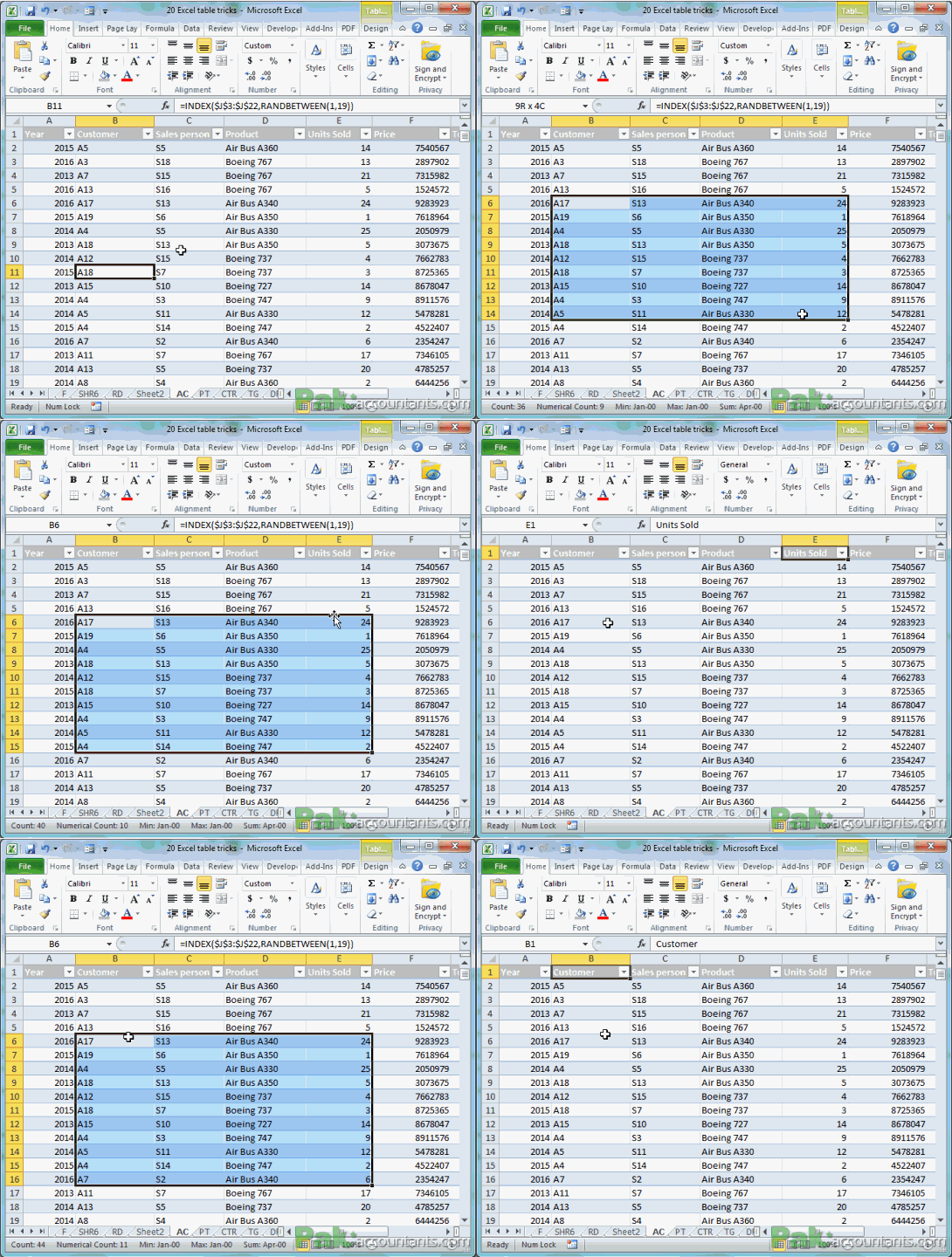
13. Jump to last row or column in the range

If you double click on the border or wall of active cell just when the cursor turn into four directions pointer then it will navigate you in the direction of border clicked i.e:

if left wall is double clicked it will navigate to far left cell in the same range in the same row. If few cells at left are empty then it will jump to last empty cell at left. If there is no filled cell at the left then it will navigate to first cell in the same row.

1. if top wall is double clicked it will navigate to top most cell in the same range in the same column. If few cells cells at above are empty then it will jump to last empty cell above. If there is no filled cell above in the same column then it will navigate to first cell in the same column.
2. If bottom wall is double clicked it will navigate to last filled cell within same range. If few cells at right are empty then it will reach the last empty cell. If there is no filled cell at right then it will not move.
3. If right wall is double clicked it will navigate to last filled cell at right within same row in the same range. If few cells at right are empty then it will reach the last empty cell. If there is no filled cell at right then it will not move.
4. If right wall is double clicked it will navigate to last filled cell  within same range in the same column downwards. If few cells below are empty then it will reach the last empty cell below. If there is no filled cell below then it will not move.

Bonus Tip – Selection using double click

Using the same technique and based on same mechanism if you press and hold Shift key then excel will not only jump cells but also make selection. This is one way of instant selection with minimal effort.

Shift + Double click cell border or wall to select to last cell in the column. At left and right to last unfilled cell. Top to bottom selects the last filled cell in the same direction. Within range and out of range has different behaviour

14. Get in edit mode and double click again and drag to make selection

Double click the cell to enter edit mode. Its an alternative to pressing F2.

Double clicking cell won’t affect the existing content of the cell as it is simply activating edit mode.

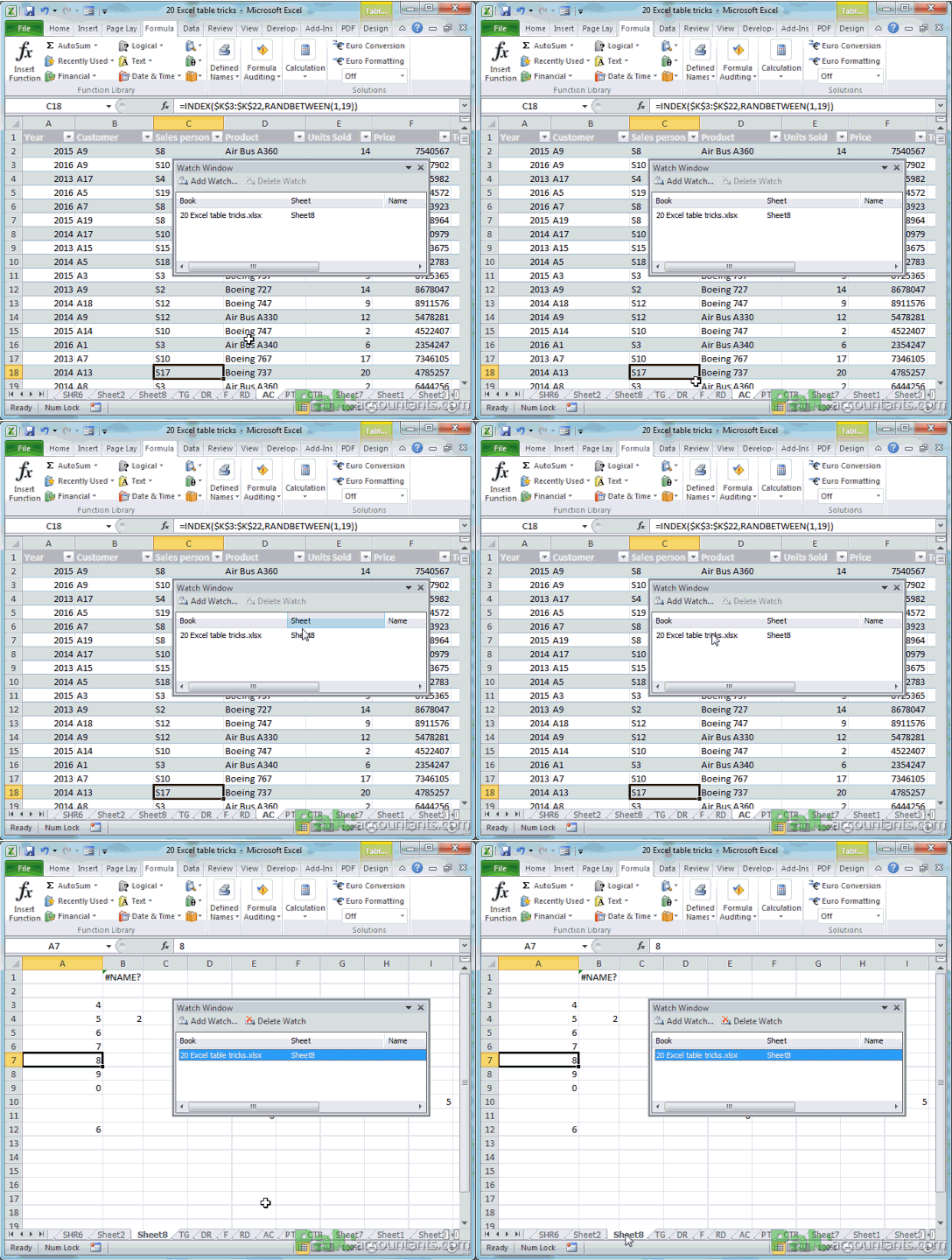
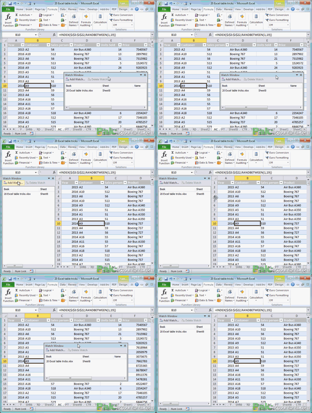
15. Double click in watch window to select that cell

If you have watch window activated and double click on any cell’s parameters then it will instantly go that cell. In the following animation the cell added to watch is on another worksheet named “Sheet 8” whereas currently active worksheet is “AC”. If cell parameters in watch window are double clicked then you will navigate to that cell

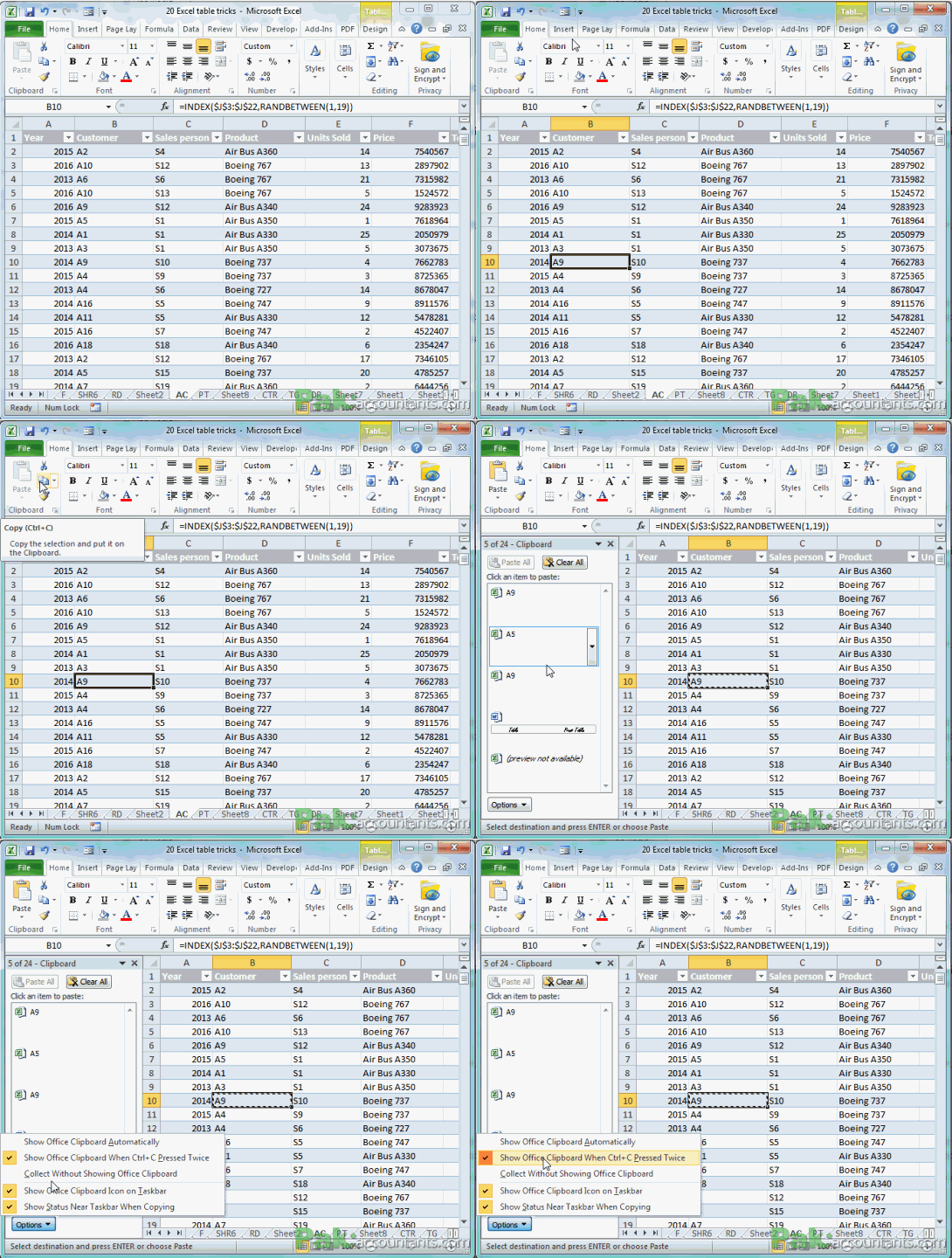
16. Show office clipboard task pane on double clicking copy button

If the option to open office clipboard on pressing Ctrl+C twice is active then pressing Copy button twice will not only copy the selected data but also kicks open the office clipboard.

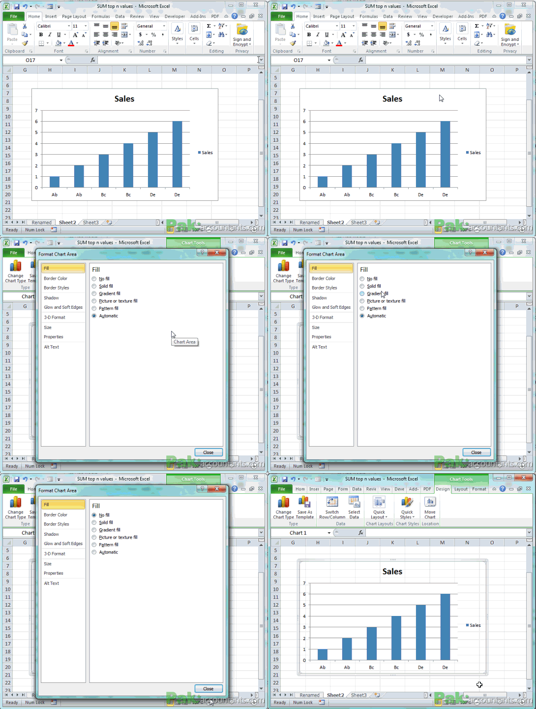
17. Double click chart to bring up properties dialogue

Although you find many of the formatting options in the contextual tab however, if you double click anywhere on chart area (not on chart items/elements) or on chart border then format options dialogue box will pop up.

Same way if you double click any element of chart then formatting options for that specific element will open and you can make adjustments as you wish.

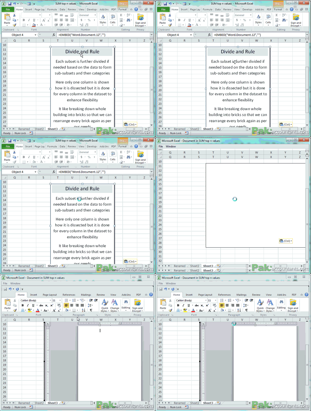
18. Double click embedded object to display respective program’s bar

If you have embedded object from other office applications like word. Then double clicking the object will put you in hybrid environment where you will be provided with the ribbon of that specific application from where the object is embedded.

Check the excel icon at top left. The Microsoft Word bar appears inside Excel to let it edit on the go. Once done click outside embedded object and you are back in Excel.

19. Double click top bar of any task pane and it will rest either left or right of the worksheet

If any task pane that is floating inside workspace, double clicking the top bar will dock the pane either at the left side of worksheet or right and saves you drag and drop arrangement of windows.

20. Insert multiple shapes easily

Press and hold Ctrl and click shape under the Insert tab>Illustrations>Shapes and it will be inserted on the worksheet and you don’t have to draw that by clicking and dragging inside work space. It works with all the shapes including text box.

But before you are able to use Ctrl key you have to draw first shape and then from the shapes options in the ribbon you can insert multiple shapes while holding Ctrl key and left click on shapes.

21. Lock drawing mode

Right click on shape and select lock drawing mode and now you can draw the same shape multiple times without coming back to insert tab. Great time saver.

22. Scroll wheel to scroll through ribbon

Normally one has to click on each tab to access the groups under each of them. However, if you hover cursor on ribbon and use scroll wheel on mouse (if yours have one) then you can scroll through tabs like a breeze.

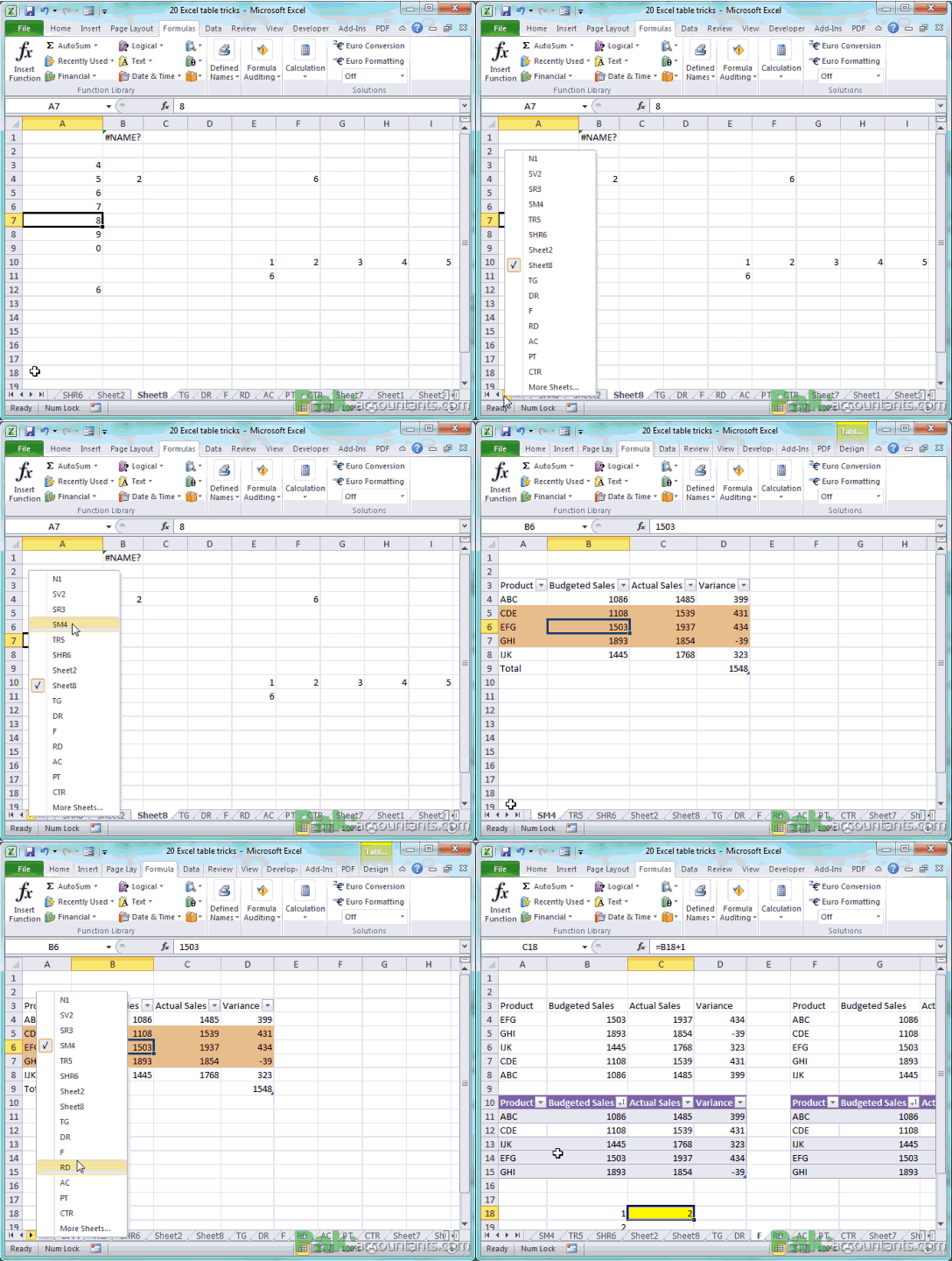
23. Right click worksheet navigation buttons to get a menu and select worksheets

This is one of my personal favourite. At times one workbook contains many worksheets and you have click navigation buttons several time to go to specific worksheet. Believe me this is tiring.

The best way is to right click on the navigation buttons and you will have a menu from which you can select the worksheet to jump to. I like jumping!

24. Select multiple worksheets by holding Shift or Ctrl key

If you have to move or copy certain worksheet to another workbook then you can move or copy multiple worksheet in one go.

If you press and hold Shift key then you will select all the worksheets between two points of selection.

If you press and hold Ctrl key then only those worksheets will be selected that are clicked.

25. Quick paste only values of whole column

If you have formula in the column to calculate certain value and later you just want values the normal course is to copy the column and use paste special to paste values in place. However, if you select the column in which you want to replace formulas with values only then right click selection border, move the selection a bit in any direction and back in its place, release right click and from the context menu select “copy here as values only”. Keyboard knuckleheads move over! 😀

26. Hold down shift key and click to select multiple rows and columns

One can make selection by single left mouse click hold and drag. However, there is a quick way to do this. Have one cell active press and hold Shift key and click another cell and immediately all the enclosed rows and columns will be selected.

27. Hold down Ctrl key to select specific cells or rows/columns

If you click and hold Ctrl key instead of shift key then it will help you make non-contiguous selection i.e. only those cells or rows / columns will be selected that you actually press on or select.

28. Move or modify formula range easily

If you apply formula then excel highlights each range with different colour. This not only help you identify what range relates to what argument in the formula but also you can extend or reduce the range or even move the range while in edit mode to quickly update the formula.

To move the range simply left click and hold on any border of range and while holding the left mouse button down drag it to another place.

To expand or contract the range you can use corners and just when mouse turns two directional pointer click and hold mouse left button and drag. It will update the range accordingly.

29. Select whole worksheet by clicking the button where rows and columns intersect

Most of Excel users know about this smart selection button. But if you don’t then it is one great alternative to Ctrl+A to select whole worksheet at once.

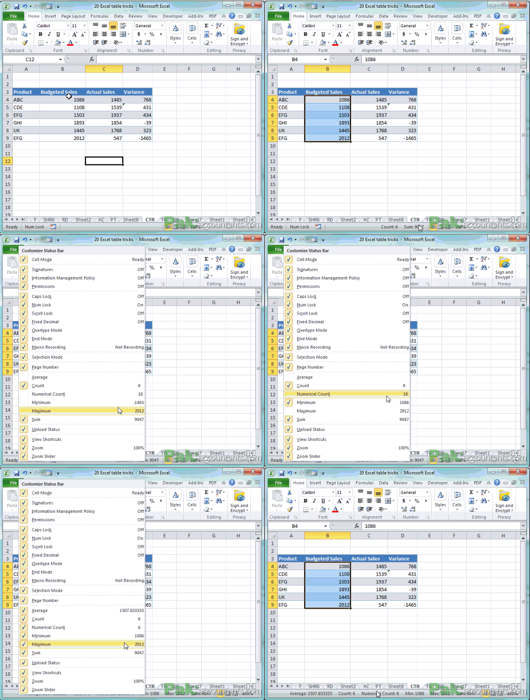
30. Right click status bar to enable multiple options like average etc.

Status bar which is located at the bottom of the excel application window is home to some of usual information user needs. For example if you select few cells then it gives you information regarding sum of numerical content, count of number of cells selected, average of numbers within selection etc. However, you can select or deselect more of such information by right clicking status bar and check/uncheck desired information.

31. Group specific worksheets’ tabs together

With multiple worksheets open within workbook. It is more comfortable if related worksheets are grouped together. To make it convenient select the worksheets you want to group together by holding Ctrl key and move the selected worksheets to be placed after particular worksheet by releasing the left mouse button.

In the following example worksheets named F, RD, AC, PT and CTR were selected using Ctrl key and then moved to be placed after DR worksheet.

32. Copy a worksheet

Simply select the worksheet or worksheets that you want to copy hold down CTRL key on the keyboard + press and hold left mouse button and drag, you will see the icon of file with plus sign in it. Release the left mouse button and it will make duplicates or copies of select worksheet(s).

33. Change Tab colors of multiple worksheets in one go

Select the worksheets the tabs of which you want to colorize differently using Shift or Ctrl key. Right click on any selected worksheet tab > Tab color and from the menu select the color. TANAA! all done in one go!

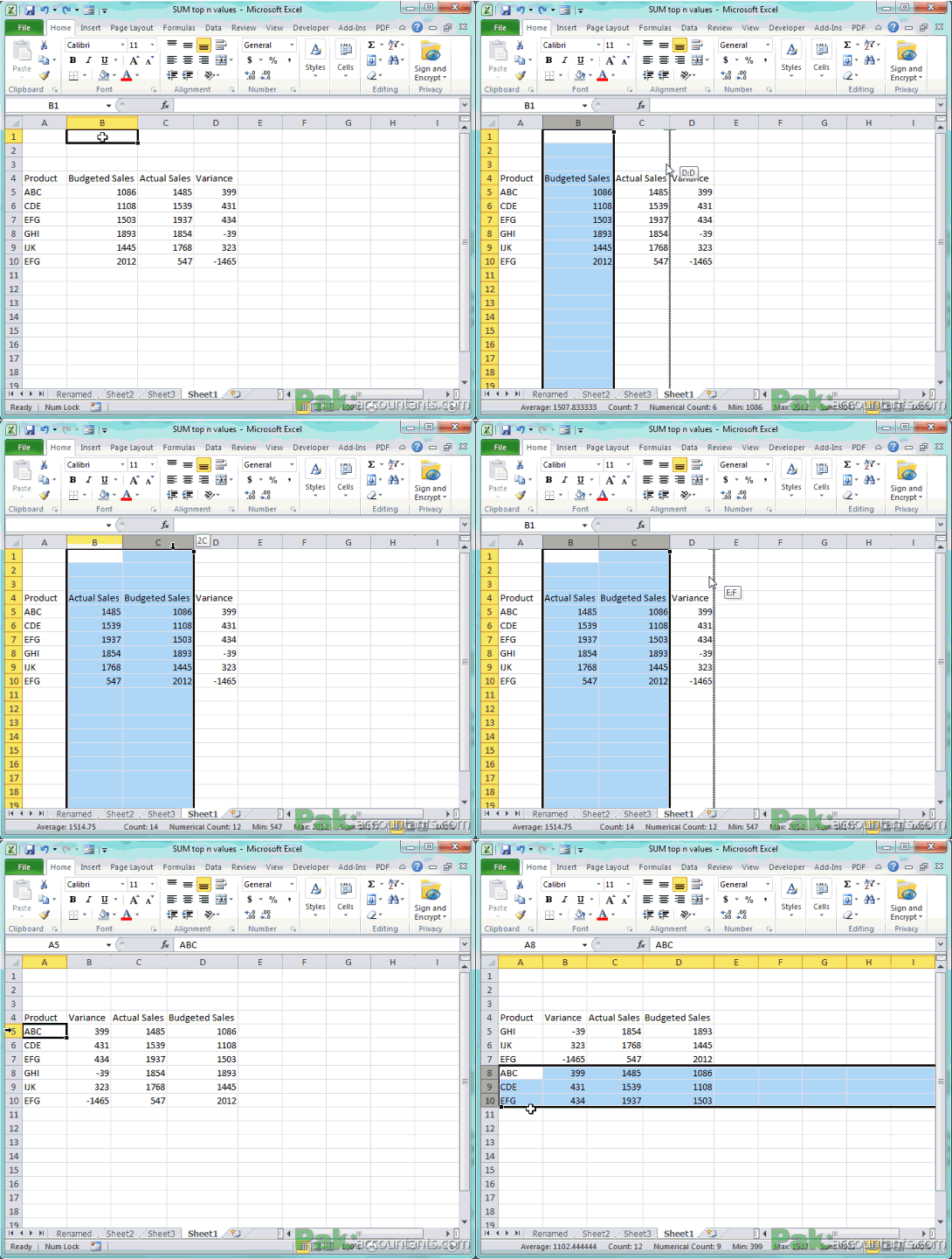
34. Move column(s) / Row(s) with ease

Select the column or row by left clicking on row/column title. Press and hold Shift key and with the mouse left click and hold on the border of selection and move in the direction where you want the column to fit. Grey margin will help you understand where on release column/row is going to be. You can do this even with multiple rows and columns at once.

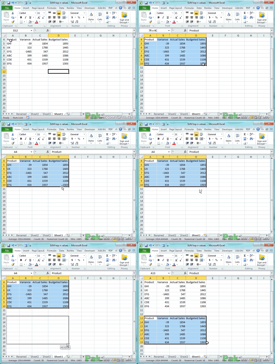
35. Quick copy selection

To quickly copy selected cells press and hold Ctrl key and drag the border of selection to get the copy and release mouse button to paste it.

36. Quick select table with/without header

Excel tables are awesome for many reasons but one cool thing is the ability to select entire table with one click. Just hover the cursor at the top left corner of the table and press left mouse button once. One first occasion it will select the enclosed data of the table. Clicking left mouse button again will select the entire table with headers.

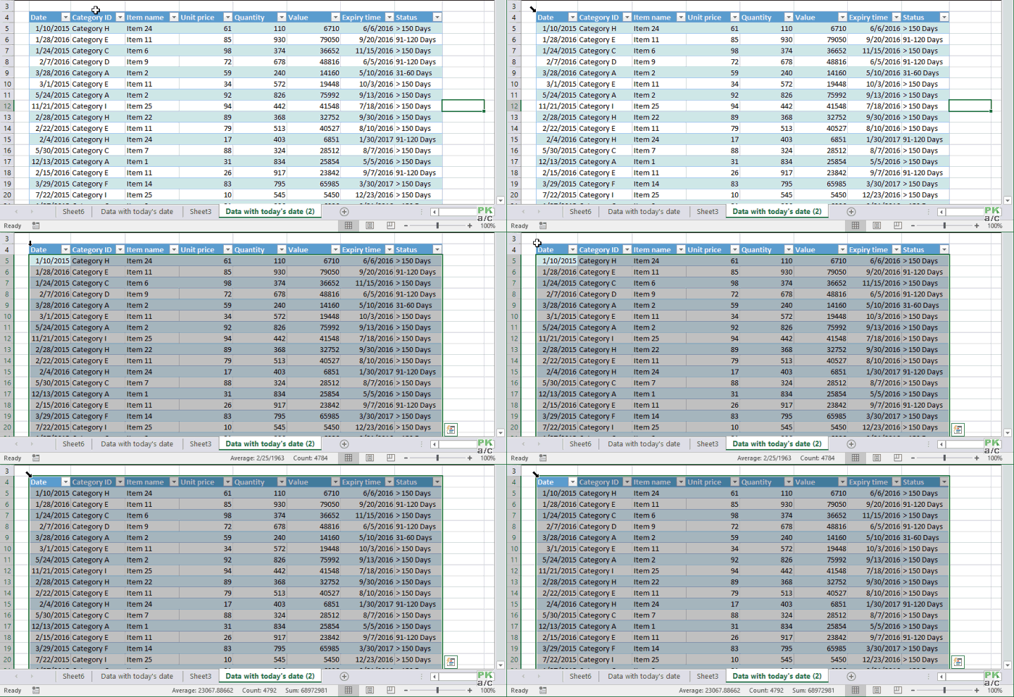
Bonus tip: Select the column/rows of table with a single click

Just like excel guides of columns and rows which you can use to select entire column or row, in Excel table, you can make selection of entire column or row with a single click by hovering the cursor at its edge.

And here you are. Am I missing any? Let me and others know about it and let’s make it a mega mouse tricks collection page. Hope you remember all of them. Only practice and using them frequently will help you remember them. But don’t forget to click on share, like and tweet.

T