10 Examples of Text to Columns || How to Split Cells/Columns in Excel

Using Excel Text to Columns Wizard to separate Delimited text [the text has some characters or delimiter, such as comma (‘,‘), tab, underscore (‘_‘), hyphen (‘–‘), at the rate (‘@‘), space (‘ ‘), etc.] into the multiple columns.

Convert Text to Columns can work for a single column only at a time, it does not work with multiple columns.

In advanced Excel, this feature is basically used to convert ‘invalid date formats to a valid date format’, convert ‘number to text’ format and ‘text to number‘ format, split a ‘delimited text into multiple columns’, etc.

There are two separate features of Convert Text to Columns:

(1) Delimited: This feature splits the text which is being joined by characters, Commas, Tabs, Spaces, Semicolons, Colons, or any other character such as a hyphen (-), underscore ( _), slash ( / ), etc.

(2) Fixed Width: This feature splits the text having a fixed width (i.e., count of characters in the text remain same in each cell) which is being joined with spaces or hyphen or underscore or slash after some fixed width.

(I). STEPS TO START TO CONVERT TEXT TO COLUMNS WIZARD

➢ Method 1: Using the Excel Shortcut

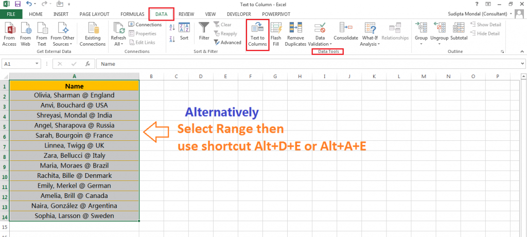
Select the data range, i.e., A2:A14 ➪ Press either Alt+D+E (sequentially press Alt, D, E) or Alt+A+E (sequentially press Alt, A, E) which will open the ‘Convert Text to Columns Wizard’.

■ Note: We had detail discussed on Excel shortcuts in separate two tutorials, suggested you read these tutorials:

80+ Excel Shortcuts with ALT Key || Best Hotkey of Keyboard Shortcuts

90+ Best Excel CTRL Shortcuts | Useful Keyboard Shortcuts |

➢ Method 2: Using the Ribbon

Select the data range, i.e., A2:A14 ➪ Go to the ‘Data‘ tab ➪ Click on ‘Text to Columns‘ under the Data Tools section ➪ ‘Convert Text to Columns Wizard‘ appears.

(II). EXAMPLES OF CONVERT TEXT TO COLUMNS WIZARD

Here we explain the usage of Text to Columns in advance excel with 10 different kinds of examples:

žžžž■ EXAMPLE 1: SPLIT FIRST NAME, LAST NAME (DELIMITER IS COMMA ‘,’) & COUNTRY NAME (DELIMITERS ARE AT THE RATE ‘@’ AND SPACE ‘ ‘)

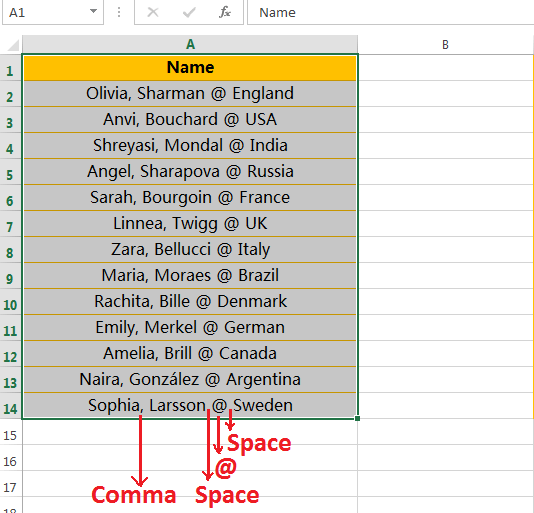
Text to Columns (Split Names and Country Names)-1

• Select the data range (A2:A14) or the entire column (Column A)

• Press either Alt+D+E (sequentially press Alt, D, E) or Alt+A+E (sequentially press Alt, A, E) which will open the ‘Convert Text to Columns Wizard‘.

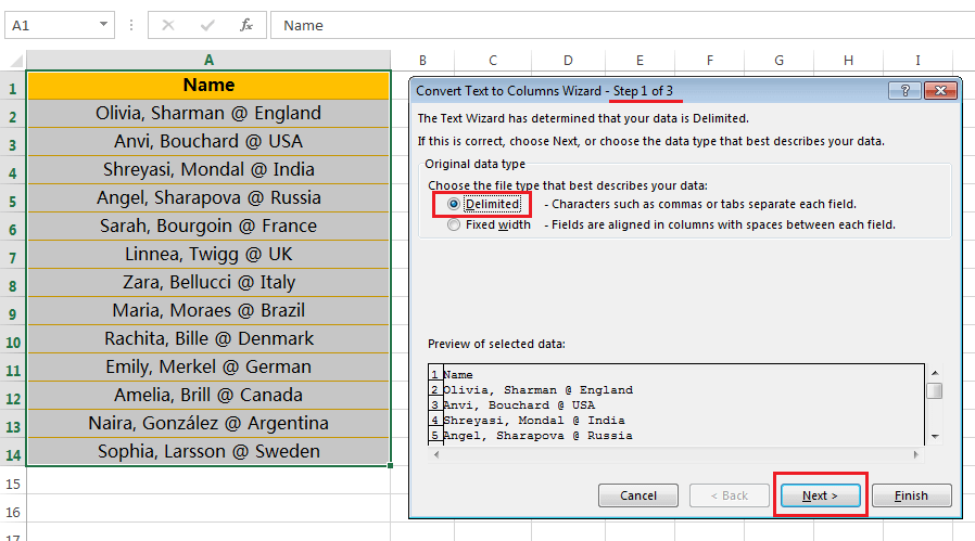
• In Step 1, select the Delimited (default option) radio button and then click Next or press Enter.

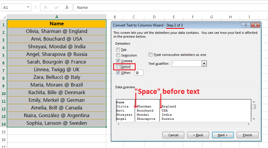
Text to Columns (Split Names and Country Names)-2

• In Step 2, select the checkboxes of ‘Comma‘, ‘Space‘ and ‘Other‘ [enter @ in the box to the right of it] as the delimiters. If there are double/triple consecutive spaces between the names, additionally select the ‘Treat consecutive delimiters as one‘ checkbox.

Then click Next or press Enter.

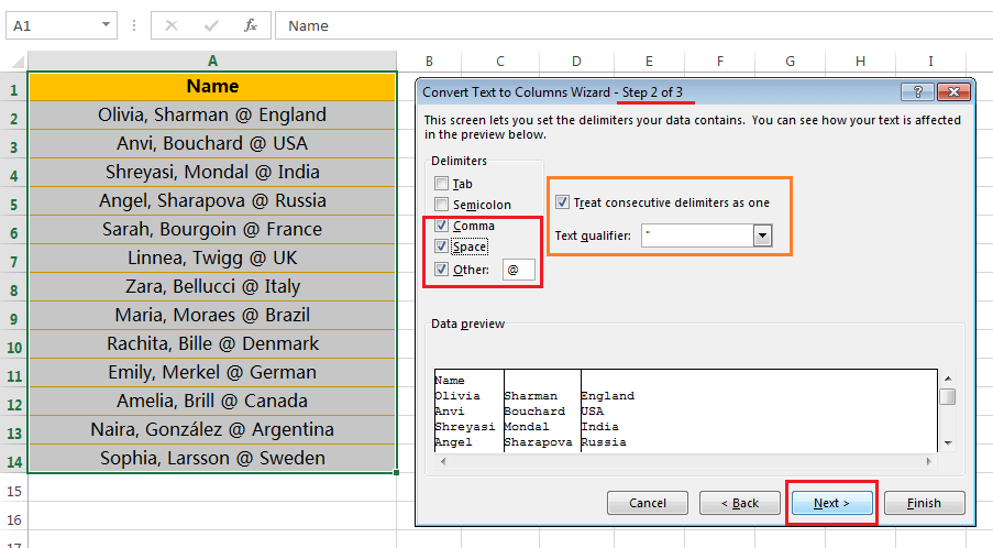
Text to Columns (Split Names and Country Names)-3

■ Note: We have noticed that there are extra spaces both before and after the ‘@’. If the ‘Space’ checkbox is unchecked then the spaces still persist in both before and after the ‘@’. We see the difference between the above and below.

Text to Columns (Split Names and Country Names)-4

• In Step 3, select the destination cell (e.g., here we select the cell B1). If we don’t select a destination cell, it would overwrite our existing database with the first name in the first column (column A), last name in the adjacent column (column B) and country name to another column adjacent to the last name column (column C). If we want to keep our original data intact, we should create a copy of the range to another place or choose a different destination cell.

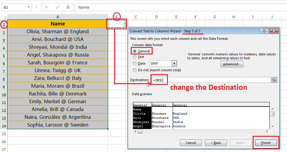
Text to Columns (Split Names and Country Names)-5

• Click Finish or press Enter on the keyboard.

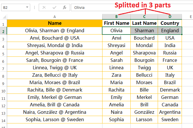
This would instantly give the results with the first name, last name and country name are split into different columns.

Text to Columns (Split Names and Country Names)-6

žžžž■ EXAMPLE 2: SPLIT DATE & TIME (DELIMITER IS SPACE ” “)

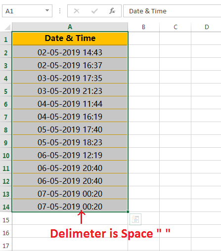
Text to column (Split Date and Time having delimiter space)-1

• Select the data range (A2:A14) or the entire column (Column A).

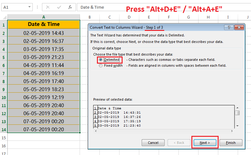
• Press either Alt+D+E (sequentially press Alt, D, E) or Alt+A+E (sequentially press Alt, A, E) which will open the ‘Convert Text to Columns Wizard‘.

• In Step 1, select the Delimited (default option) radio button and then click Next or press Enter.

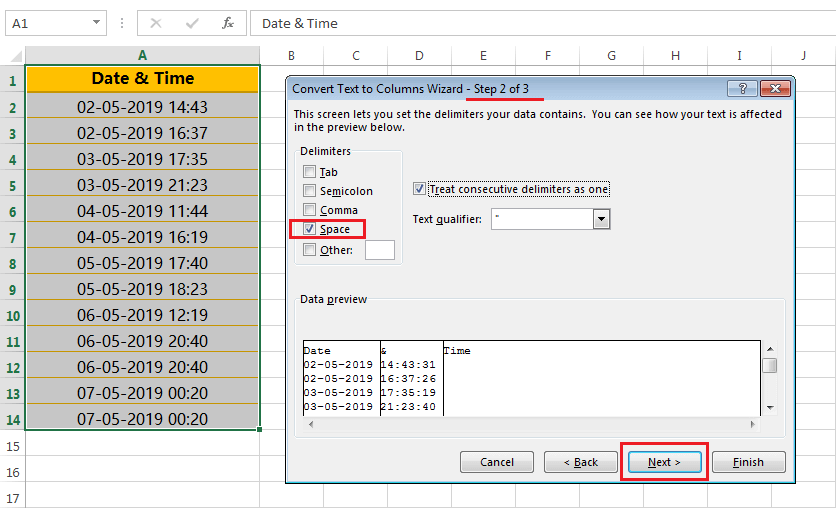
Text to column (Split Date and Time having delimiter space)-2

• In Step 2, select only the checkbox ‘Space‘. As mentioned above, if there are multiple consecutive spaces as a delimiter, also select the ‘Treat consecutive delimiters as one‘ option.

Then click Next or press Enter.

Make sure that other checkboxes must be unchecked (if any).

Text to column (Split Date and Time having delimiter space)-3

• In Step 3, select the new destination cell (e.g., Here select B1). If we don’t select a new destination cell, it would overwrite the existing dataset – such as the date in the first column (column A) and time in the adjacent column (column B). If we want to keep our original data intact, we should create a copy of the range to another place or choose a different destination cell.

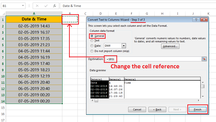
Text to column (Split Date and Time having delimiter space)-4

• Click Finish or press Enter on the keyboard.

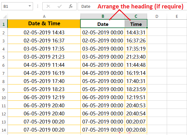
This would instantly give the results with the date in one column and time in another column. Arrange the subject heading accordingly.

Text to column (Split Date and Time having delimiter space)-5

For data preparation, we should need to arrange the date format to a valid date format in Excel such as ‘dd-mmm-yy‘ (or any other format).

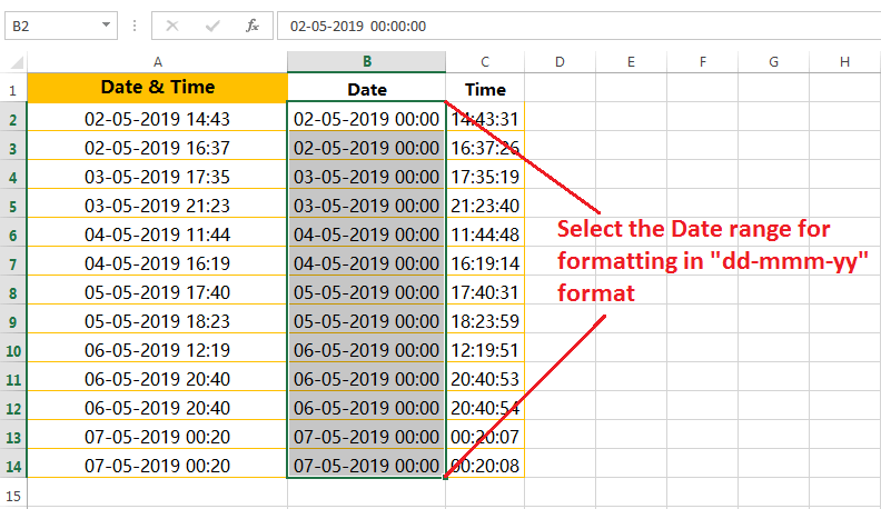
Text to Columns (Formatting of dates in a valid format)-1

We can follow any of the following methods:

(01) Using the Excel Shortcut

Select the date range B2:B14 ➪ Then press Ctrl+Shit+#. All are arranged in a valid date format.

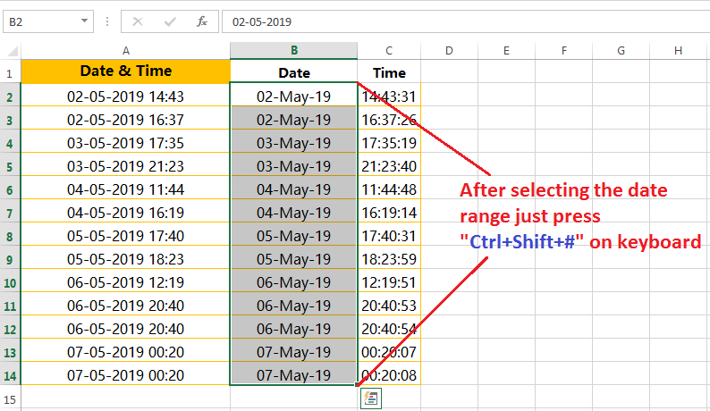
Text to Columns (Formatting of dates in a valid format)-2

(02) Using the ‘Format Cells’ Dialog Box Via Excel Shortcut

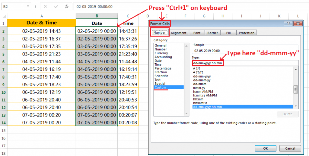
Equivalently, select the data range B2:B14 ➪ then press Ctrl+1 which will open the ‘Format Cells‘ dialog box ➪ Go to the ‘Custom’ option under the ‘Number’ tab ➪ On the right side, mentioned a valid date format like ‘dd-mmm-yy‘ under the ‘Type‘ section.

Text to Columns (Formatting of dates in a valid format)-3

(03) Using the Format Cells Dialog Box Via the Ribbon

Alternatively, select the data range B2:B14 ➪ Go to the Home tab ➪ Either click on the Alignment dialog box launcher, a small square, is located at the right side corner of the ‘Alignment‘ section or click on the Number dialog box launcher, a small square, is located at the right side corner of the ‘Number‘ section.

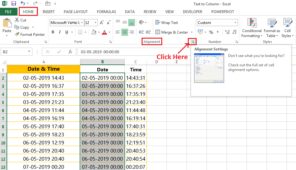
Text to Columns (Formatting of dates in a valid format)-4

As a result, the ‘Format Cells’ dialog box opens ➪ Select the ‘Custom’ option under the ‘Number’ tab ➪ On the right side, input a valid date format such as ‘dd-mmm-yy’ under the ‘Type‘ section.

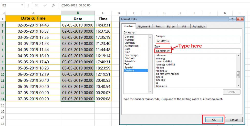
Text to Columns (Formatting of dates in a valid format)-5

Finally, press OK or press Enter on the keyboard. We get the result in the desired format as shown as below:

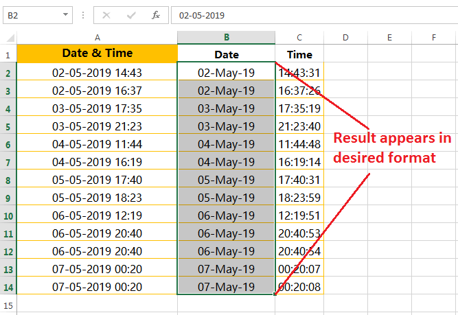
Text to Columns (Formatting of dates in a valid format)-6

■ Note: We had detail discussed on How to Change Valid Excel Date Format in a separate tutorial, suggested you read this tutorial: BEST 05 WAYS: HOW TO CHANGE DATE FORMAT IN EXCEL?

[/su_box]

žžžž■ EXAMPLE 3: CONVERT INVALID DATE FORMATS TO VALID DATE FORMATS

Sometimes we get the lists of invalid date formats during data preparation and always we would like to convert these invalid dates to valid date formats by using the following steps:

• Select the data range (A2:A11) or the entire column (Column A)

• Press either Alt+D+E (sequentially press Alt, D, E) or Alt+A+E (sequentially press Alt, A, E) which will open the ‘Convert Text to Columns Wizard‘.

• In Step 1, select the Delimited (default option) radio button and then click Next or press Enter.

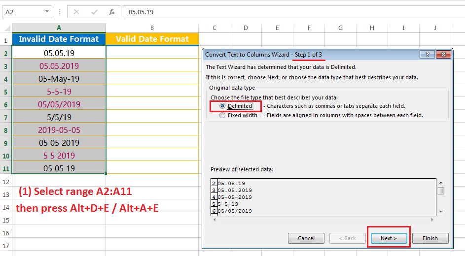
Text to Columns (Convert Invalid Date Formats to Valid Date Formats)-1

• In Step 2, please notice that all the checkboxes should be unchecked if checked any. Then click on Next or press Enter.

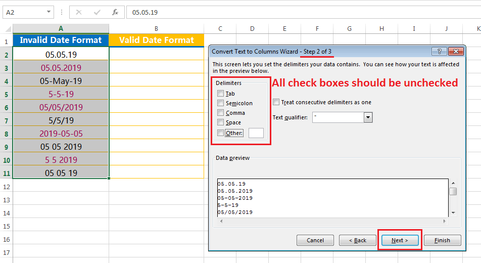
Text to Columns (Convert Invalid Date Formats to Valid Date Formats)-2

• In Step 3, select the new destination cell (e.g., in this case, we select the cell B2) to avoid overwriting the existing data set.

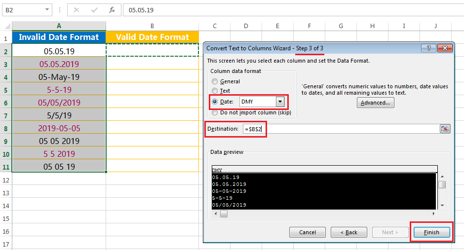
Text to Columns (Convert Invalid Date Formats to Valid Date Formats)-3

• Click ‘Finish’ or press Enter on the keyboard.

This would instantly convert the invalid date format to a valid date format.

Text to Columns (Convert Invalid Date Formats to Valid Date Formats)-4

žžžž■ EXAMPLE 4: SPLIT DATES IN THE DAYS, MONTHS & YEARS (DELIMITER IS HYPHEN “-“)

Sometimes we require to split the dates into days, months and years separately. We can do this using the following steps:

• Select the data range (A2:A14) or the entire column (Column A)

Text to Columns (Split dates in the days, months and years having delimiter hyphen)-1

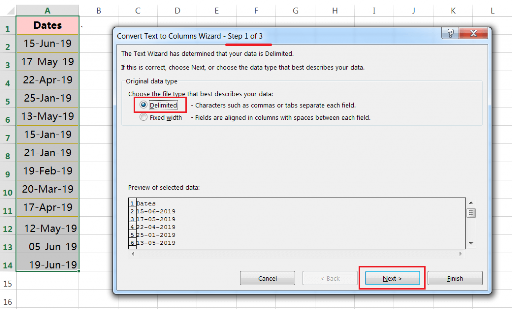
• In Step 2, select the only checkbox ‘Other‘ and enter a hyphen (-) in the box to the right of it. Please note that the hyphen is used here as the delimiter. Click Next or press Enter.

Make sure that other checkboxes should be unchecked (if any).

Text to Columns (Split dates in the days, months and years having delimiter hyphen)-2

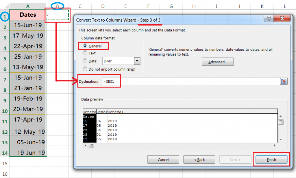
• In Step 3, select the destination cell (i.e., B1) to avoid the overwriting of existing data.

• Click ‘Finish‘ or press Enter on the keyboard.

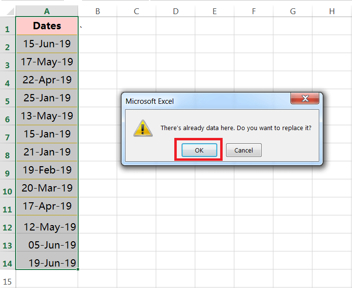
Text to Columns (Split dates in the days, months and years having delimiter hyphen)-3

• A Microsoft Excel Warning dialog box appears and confirming us do we want to replace the existing data? Click OK or press Enter to proceed.

Text to Columns (Split dates in the days, months and years having delimiter hyphen)-4

This would instantly split the days, months and years into different columns. Arrange the subject heading accordingly.

Text to Columns (Split dates in the days, months and years having delimiter hyphen)-5

žžžž■ EXAMPLE 5: JOIN DAYS, MONTHS & YEARS TO FORM VALID DATE FORMATS (DELIMITER IS SLASH “/”)

It is a very common problem found in Data preparation how making a valid date format by joining the day, month and year respectively. We can do with the following steps:

(01) To use CONCATENATE() function joining the DAYS, MONTHS and YEARS with delimiter slash ‘/’.

(02) To use ‘Paste Special’ to convert the formulas into values.

(03) Finally, using the ‘Convert Text to Columns wizard’ to convert invalid date formats to valid date formats.

(01) TO USE CONCATENATE() FUNCTION JOINING THE DAYS, MONTHS & YEARS WITH DELIMITER SLASH ‘/’

• In Step 1, we use the CONCATENATE function to join the dates, months and years.

Apply an equality ‘= ‘ sign in cell D2 and then type a few characters of ‘con…..’. Excel suggests different functions starting with ‘CON‘. Select CONCATENATE from the drop-down list and press the ‘Tab‘ key on the keyboard simultaneously. As a result, the CONCATENATE syntax appears with open parenthesis.

Text to column(Join days, months and years to form valid date formats)-1

• We should take care of joining the criteria

(i) First select the cell with a day (i.e., C2) in the CONCATENATE function and put a comma (,) to close the text1.

Use a delimiter slash (/) in the double quotes and put a comma (,) after that to close the text2.

(ii) Then select the cell with a month (i.e., B2) and put a comma (,) to close the text3.

Use a delimiter slash (/) in the double quotes and put a comma (,) after that to close the text4.

(iii) Finally, select the cell with a year (i.e., A2) and press ‘Enter’.

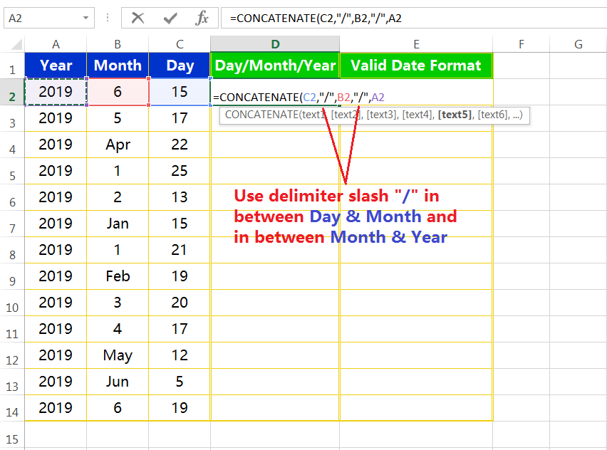
Text to column(Join days, months and years to form valid date formats)-2

• So the complete formula is =CONCATENATE(C2,”/”, B2,”/”, A2) and returns the result. Copy the formula till the end of the range.

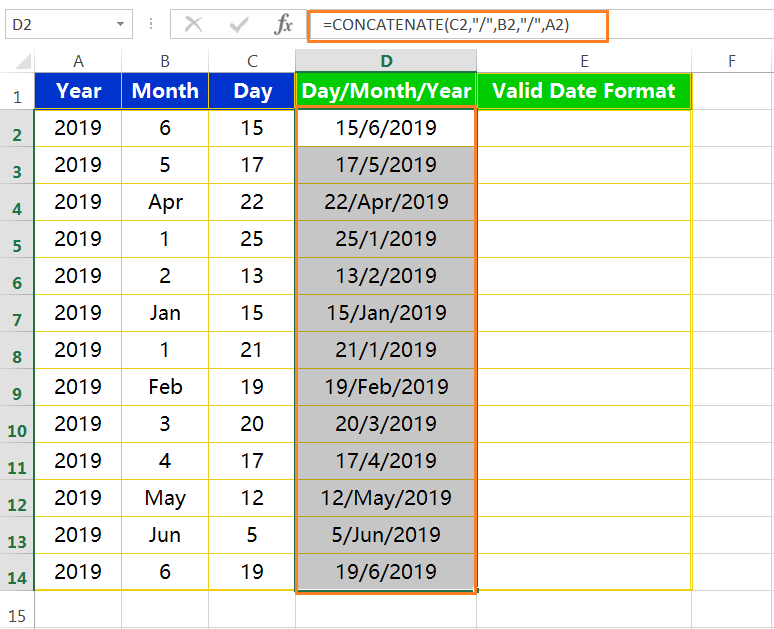
Text to column(Join days, months and years to form valid date formats)-3

(02) TO USE ‘PASTE SPECIAL’ TO CONVERT THE FORMULAS INTO VALUES

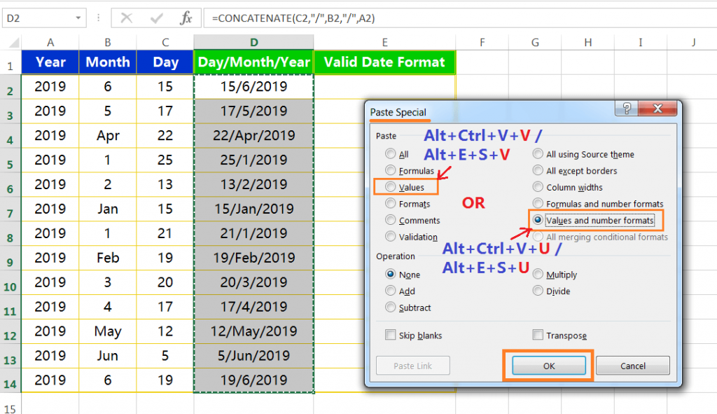
The next step converts the formula into values with the help of the Paste Special dialog box. We can follow any of the following methods:

➢ Method 1: Copy the range (D2:D14) ➪ press Alt+E+S+U (sequentially press Alt, E, S, U) or Alt+Ctrl+V+U (sequentially press Alt+Ctrl+V, U) to select the ‘Values and number formats’ option ➪ Press Enter or click OK. As result, the entire range would instantly convert formulas into values.

➢ Method 2: or press Alt+E+S+V (sequentially press Alt, E, S, V) or Alt+Ctrl+V+V (sequentially press Alt+Ctrl+V, V) to select the ‘Values’ option ➪ Press Enter or click OK. As result, the entire range would instantly convert formulas into values.

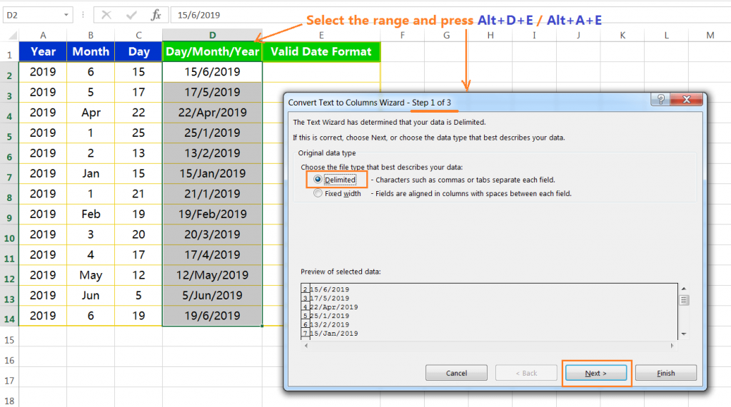
Text to column(Join days, months and years to form valid date formats)-4

(03) USING THE ‘CONVERT TEXT TO COLUMNS WIZARD’ TO CONVERT INVALID DATE FORMATS TO VALID DATE FORMATS

• Select the data range (A2:A11) or the entire column (Column A)

• Press either Alt+D+E (sequentially press Alt, D, E) or Alt+A+E (sequentially press Alt, A, E) which will open the ‘Convert Text to Columns Wizard‘.

• In Step 1, select the Delimited (default option) radio button and then click Next or press Enter.

Text to column(Join days, months and years to form valid date formats)-5

• In Step 2, please notice that all the checkboxes should be unchecked if checked any. Then click Next or press Enter.

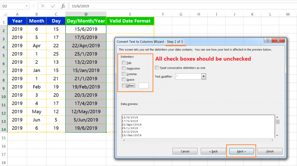
Text to column(Join days, months and years to form valid date formats)-6

• In Step 3, select the destination cell (i.e., E2) to avoid the overwriting of existing data.

Then select the Date checkbox.

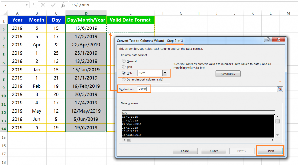
Text to column(Join days, months and years to form valid date formats)-7

Click ‘Finish‘ or press Enter on the keyboard.

This would instantly convert invalid date formats to valid date formats.

Text to column(Join days, months and years to form valid date formats)-8

žžžž■ EXAMPLE 6: SPLIT TEXT INTO YEARS, HOST NAMES & WINNER TEAM (DELIMITERS ARE HYPHEN “-” & UNDERSCORE “_”)

Both the delimiters hyphen ‘-‘ and underscore ‘_’ didn’t use at a time in Convert Text to Columns Wizard. Because these delimiters are used in the ‘Other’ box, but the Other box only allows a single delimiter at a time. So in that case, we should apply the ‘Convert Text to Columns Wizard’ twice to split the delimiters.

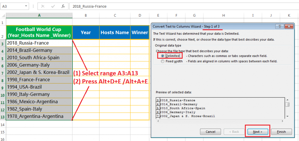
• Select the data range (A3:A13) or the entire column (Column A).

• Press either Alt+D+E (sequentially press Alt, D, E) or Alt+A+E (sequentially press Alt, A, E) which will open the ‘Convert Text to Columns Wizard‘.

• In Step 1, select the Delimited (default option) radio button and then click Next or press Enter.

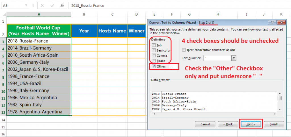
Text to column (Split text into Years, Hosts Name & Winner Team having delimiter hyphen and underscore)-1

• In Step 2, select the only checkbox ‘Other’ and enter an underscore ‘_’ in the box to the right of it. Please note that the underscore is used here as a delimiter. Click Next or press Enter.

Make sure that other checkboxes should be unchecked (if any).

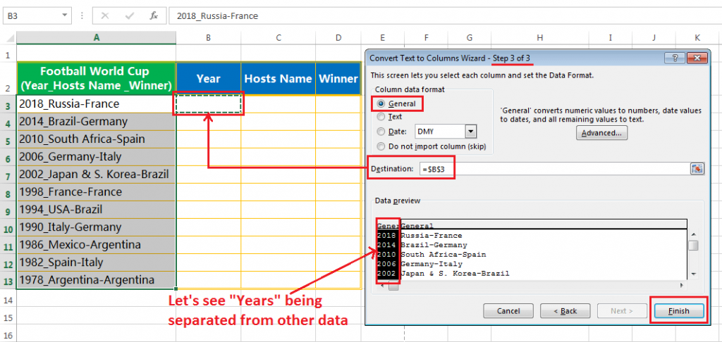
Text to column (Split text into Years, Hosts Name & Winner Team having delimiter hyphen and underscore)-2

• In Step 3, select the destination cell (i.e., B2) to avoid the overwriting of existing data.

Click on ‘Finish‘ or press Enter on the keyboard.

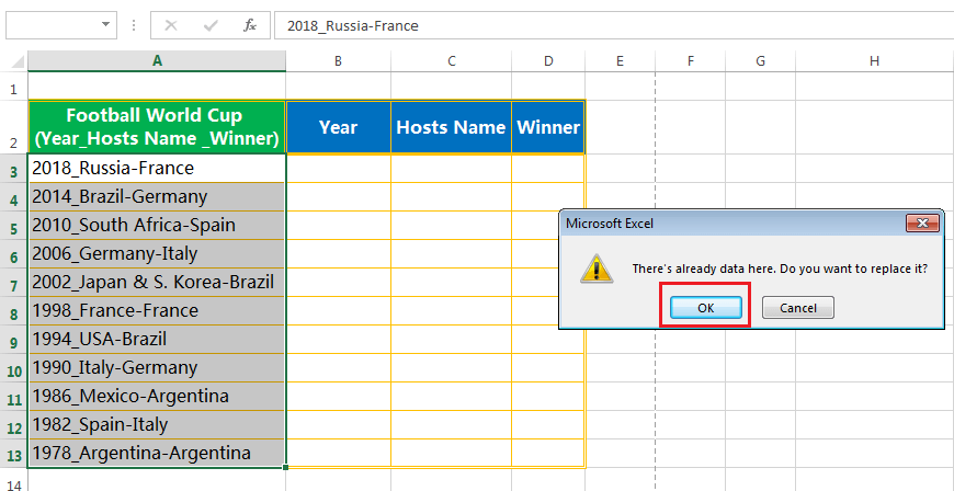
Text to column (Split text into Years, Hosts Name & Winner Team having delimiter hyphen and underscore)-3

• A Microsoft Excel Warning dialog box appears and confirming us do we want to replace the existing data? Click OK or press Enter to proceed.

This would instantly split the Year from given data.

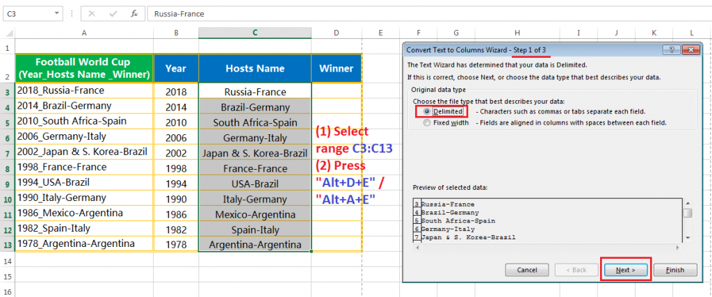
Text to column (Split text into Years, Hosts Name & Winner Team having delimiter hyphen and underscore)-4

Repeat the same process to split the Host Name and Winner Team.

• Select the data range (C3:C13) or the entire column (Column C)

• Press either Alt+D+E (sequentially press Alt, D, E) or Alt+A+E (sequentially press Alt, A, E) which will open the ‘Convert Text to Columns Wizard‘.

• In Step 1, select the Delimited (default option) radio button and then click Next or press Enter.

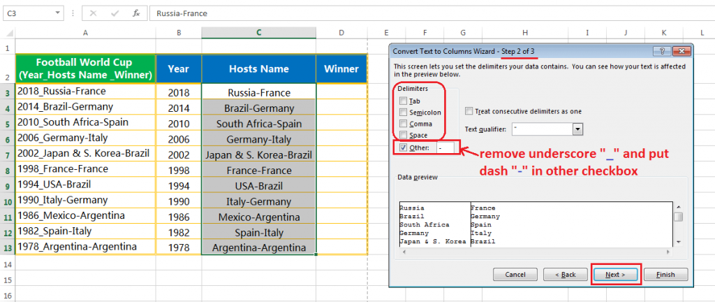
Text to column (Split text into Years, Hosts Name & Winner Team having delimiter hyphen and underscore)-5

• In Step 2, select the only checkbox ‘Other’ and enter a hyphen ‘-‘ in the box to the right of it. Please note that the hyphen is used here as the delimiter. Click on Next or press Enter.

Make sure that other checkboxes should be unchecked (if any).

Text to column (Split text into Years, Hosts Name & Winner Team having delimiter hyphen and underscore)-6

• In Step 3, keep the default destination cell (e.g., C2), no need to change the destination cell.

• Click ‘Finish‘ or press Enter on the keyboard.

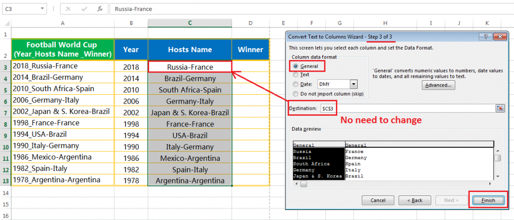
Text to column (Split text into Years, Hosts Name & Winner Team having delimiter hyphen and underscore)-7

• A Microsoft Excel Warning dialog box appears and confirming us do we want to replace the existing data? Click OK or press Enter to proceed.

Text to column (Split text into Years, Hosts Name & Winner Team having delimiter hyphen and underscore)-8

• This would instantly split the Hosts name and Winner Team into two parts.

Text to column (Split text into Years, Hosts Name & Winner Team having delimiter hyphen and underscore)-9

■ EXAMPLE 7: CONVERT TEXT TO NUMBERS

Sometimes imported data from databases or other file formats (like CSV), the numbers are converted into text format.

It mainly happens in two ways:

• Having an apostrophe before the number. This leads to the number being treated as text.

• Getting numbers as a result of text functions such as LEFT, RIGHT, MID, CONCATENATE.

The problem arises with these numbers (which are in text format) as those numbers are basically ignored by Excel formulas such as VLOOKUP, SUM, AVERAGE, SUMIFS, etc.

Let’s start with an example database as shown below:

Text to column(Convert Text to Numbers)-1

[su_box title=”HOW DO WE IDENTIFY A NUMBER IS EITHER IN GENERAL FORMAT OR IN TEXT FORMAT?” style=”noise” box_color=”#7b204b”]

It is very simple to identify a number is either in general format or text format in the following ways:

Identify General Format:

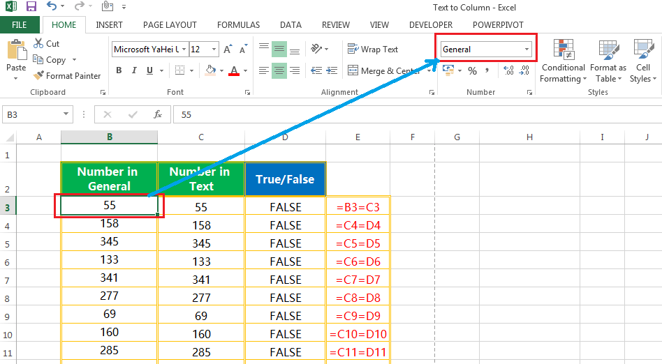
Text to column(Convert Text to Numbers)-2

Identify Text Format:

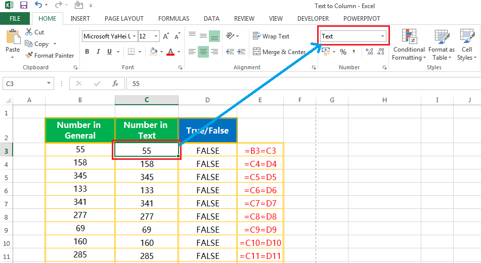
Text to column(Convert Text to Numbers)-3

[/su_box]

Steps to Start:

• Select the data range (C3:C12) or the entire column (Column C)

• Press either Alt+D+E (sequentially press Alt, D, E) or Alt+A+E (sequentially press Alt, A, E) which will open the ‘Convert Text to Columns Wizard‘.

• In Step 1, select the Delimited (default option) radio button and then click Next or press Enter.

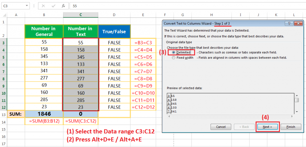
Text to column(Convert Text to Numbers)-4

• In Step 2, please notice that all the checkboxes should be unchecked if checked any. Then click Next or press Enter.

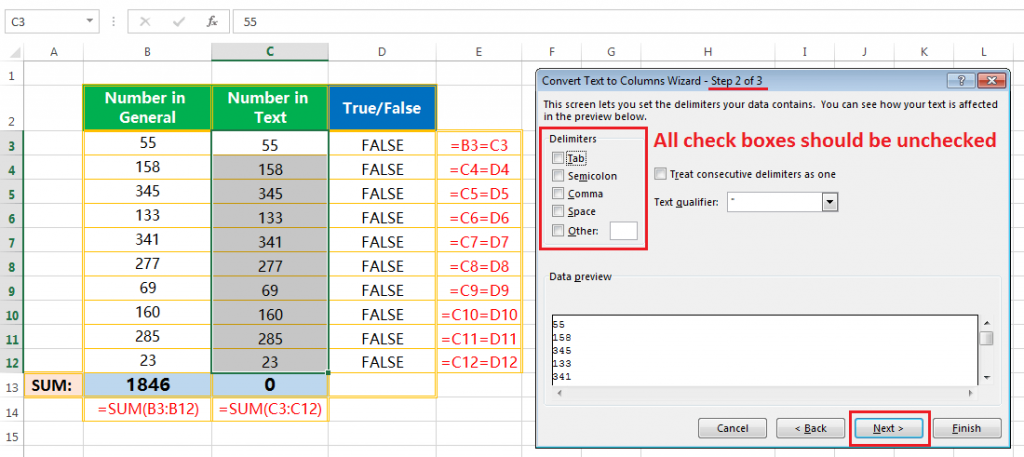
Text to column(Convert Text to Numbers)-5

• In Step 3, keep the default destination cell (i.e., C3), no need to change the destination cell. The Column data format should be in ‘General’ (otherwise select the General checkbox).

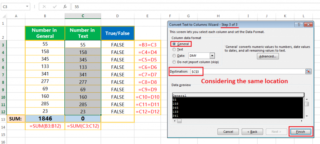
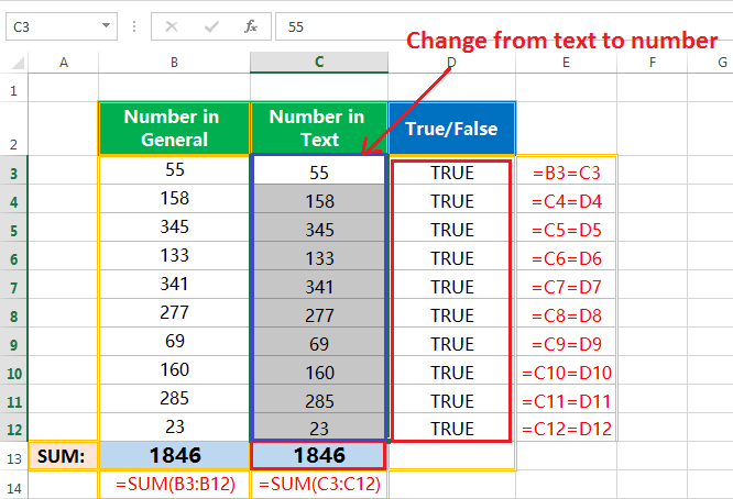
Text to column(Convert Text to Numbers)-6

Click ‘Finish’ or press Enter on the keyboard.

This would instantly convert the text to the number. Therefore, the formula works henceforth.

Text to column(Convert Text to Numbers)-7

■ EXAMPLE 8: CONVERT NUMBER TO TEXT

• After putting a large number (12 or more digits) in a cell the general format uses scientific (exponential) notation like 9333E+15.

• If we convert this number to number format the last digit has been modified.

So in these cases, we would like to convert the number to text.

Text to column(Convert Number to text)-1 To overcome the situation, we first change the cell format in text format by using ‘Convert Text to Columns Wizard’.

• Select the data range (B2:B13) or the entire column (Column B).

• Press either Alt+D+E (sequentially press Alt, D, E) or Alt+A+E (sequentially press Alt, A, E) which will open the ‘Convert Text to Columns Wizard‘.

• In Step 1, select the Delimited (default option) radio button and then click Next or press Enter.

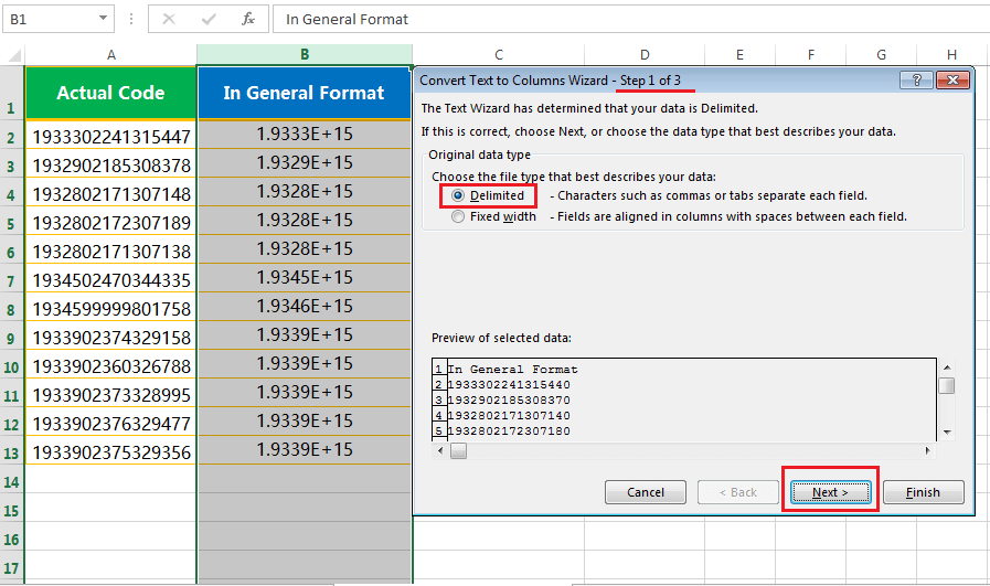
Text to column(Convert Number to text)-2

• In Step 2, please notice that all the checkboxes should be unchecked if checked any. Then click Next or press Enter.

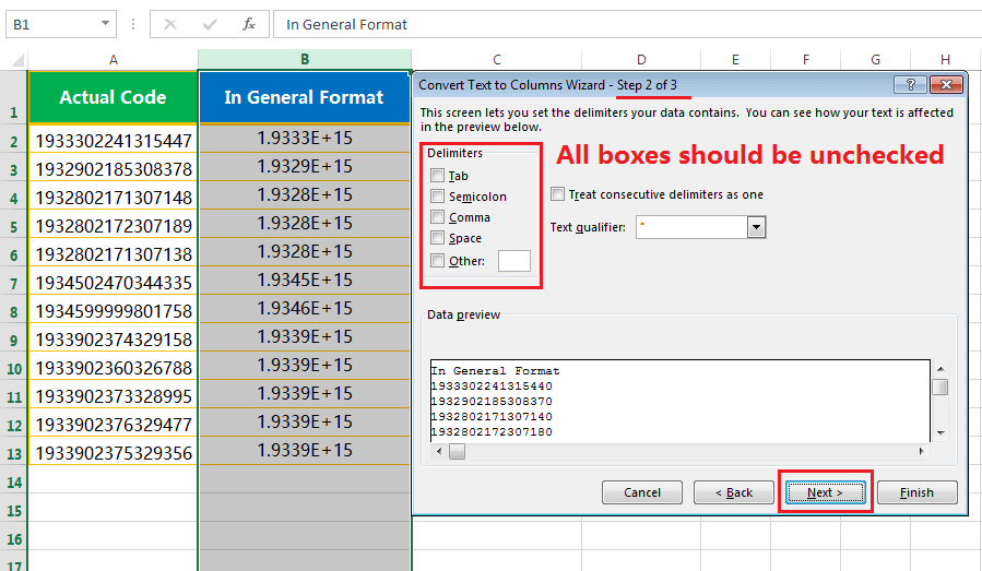
Text to column(Convert Number to text)-3

• In Step 3, keep the default destination cell (e.g., B2), no need to change the destination cell. The Column data format should be selected in the ‘Text‘ checkbox.

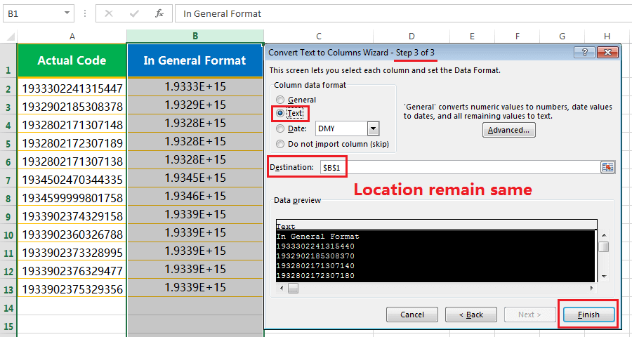
Text to column(Convert Number to text)-4

Click ‘Finish’ or press Enter on the keyboard.

This would instantly give the results in text format. Arrange the subject heading accordingly.

Text to column(Convert Number to text)-5

■ EXAMPLE 9: EXTRACT FIRST / LAST FEW CHARACTERS OF A FIXED WIDTH TEXT/STRING

If we require to extract the first 4 characters and last 5 characters from a fixed-width text /string, then we go for the Fixed width option instead of the Delimited (default) option in the Convert Text to Columns Wizard.

Suppose we have codes having the same characters (we can apply the LEN function for checking the characters count if require) and we need to extract the first 4 characters and the last 5 characters from it.

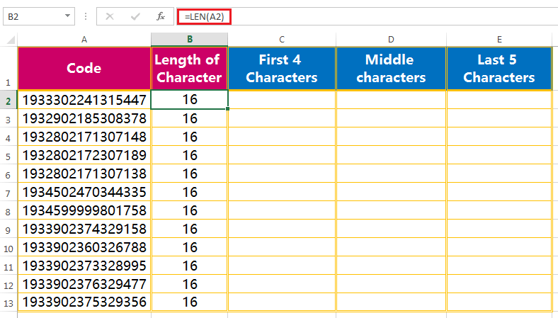
Text to column (Extract Few Characters of a fixed width text or String)-1

Here are the steps to quickly extract the characters from a text/string using the Convert Text to Columns Wizard:

• Select the data range (A2:A13) or the entire column (Column A)

• Press either Alt+D+E (sequentially press Alt, D, E) or Alt+A+E (sequentially press Alt, A, E) which will open the ‘Convert Text to Columns Wizard‘.

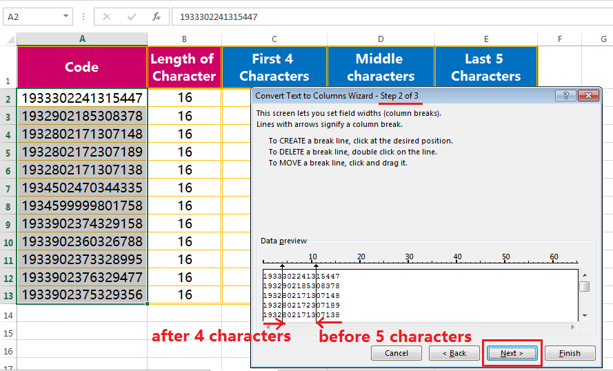
• In Step 1, we select Fixed Width (don’t select ‘Delimited’) and then click Next or press Enter.

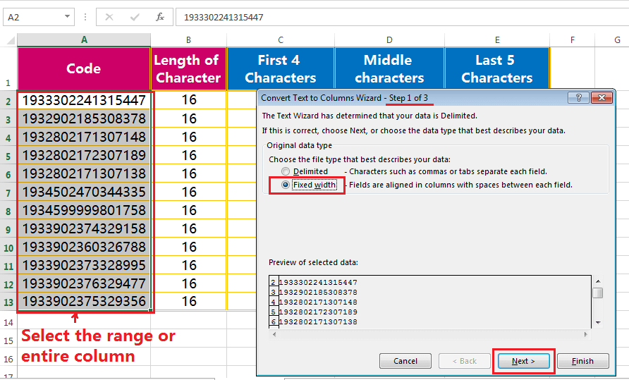
Text to column (Extract Few Characters of a fixed width text or String)-2

• In Step 2, in the Data preview section, click after the first 4 characters in the text to create a break-line and then create another break-line to click from the last 5 characters before.

Finally, click on Next or press Enter.

■ Note:

➢ If wrongly placed a break-line anywhere in the text, we can delete/remove it by double-clicking on it.

➢ If we want to move it to another place, simply click and drag it to another location.

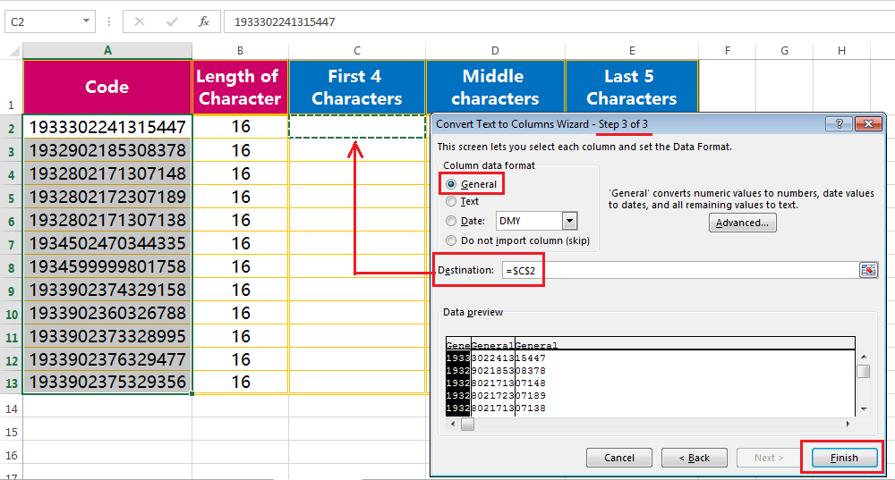
Text to column (Extract Few Characters of a fixed width text or String)-3

• In Step 3, select a new destination cell (e.g., here we select the cell C2) to avoid the overwriting of existing data.

Make sure that the Column data format ‘General’ should be checked.

Click ‘Finish‘ or press Enter on the keyboard.

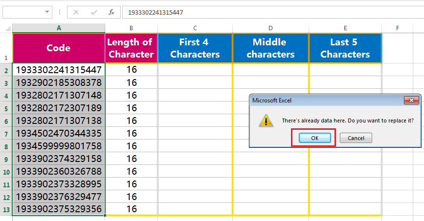
Text to column (Extract Few Characters of a fixed width text or String)-4

• A Microsoft Excel Warning dialog box appears and confirming us do we want to replace the existing data? Click OK or press Enter to proceed.

Text to column (Extract Few Characters of a fixed width text or String)-5

• This would split the data into three parts – the first part contains 4 characters (required), the last part contains 5 characters (required) and the middle part contains rest characters (not required). We should delete this column with the Excel shortcut Ctrl + minus (-).

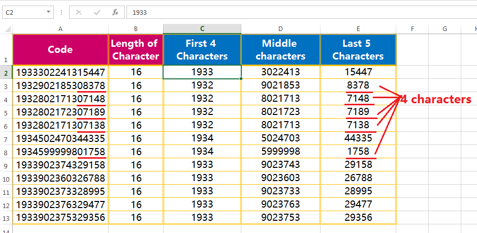
Text to column (Extract Few Characters of a fixed width text or String)-6

If we notice carefully, in some cases leading zero is missing after splitting. We can add this with a separate method.

[su_box title=”HOW DO WE ADD LEADING ZERO(S) OF ANY NUMBER?” style=”noise” box_color=”#533a76″]

Please keep in mind that the number with starting zero value is omitted by default in Excel. For this reason, we find some numbers having 4 digits after splitting in spite of 5 digits.

If it is the mandates to keep the last 5 digits intact, obviously we need to add zero before the number. This is done more dynamically with the TEXT function.

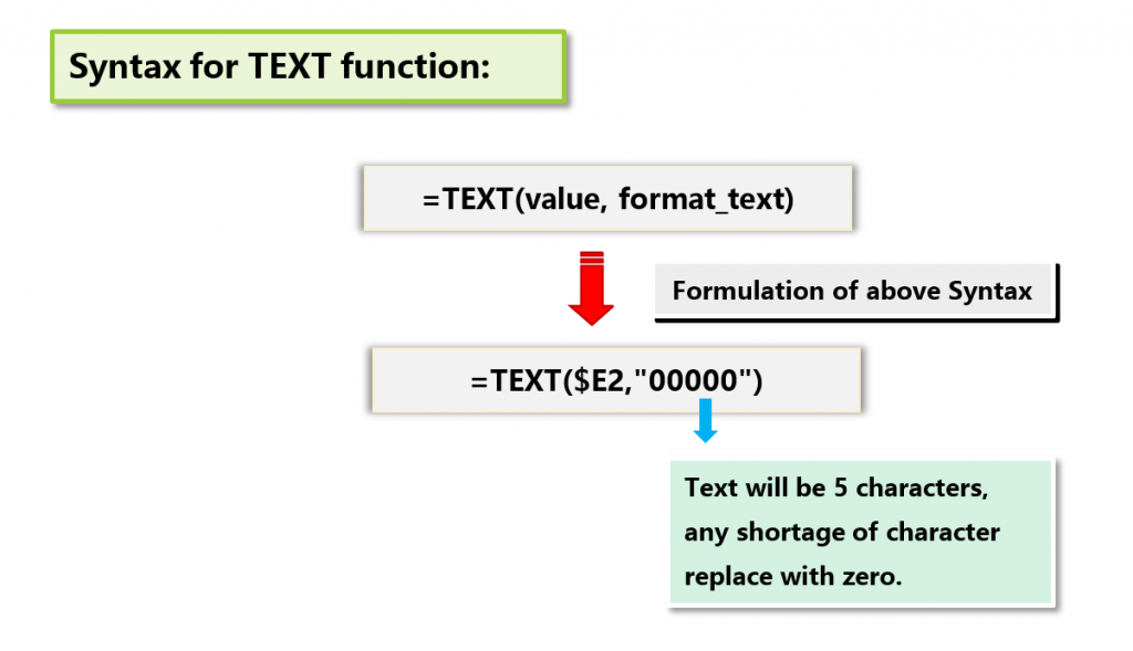
Text to Columns (Syntax of TEXT function)

In the given example, the TEXT function is applied in a separate column and within the TEXT syntax using five-times zeros in double quotation likes ‘00000‘ which refers that our text value should be 5 characters, any shortage of character it replaces with leading zero(s).

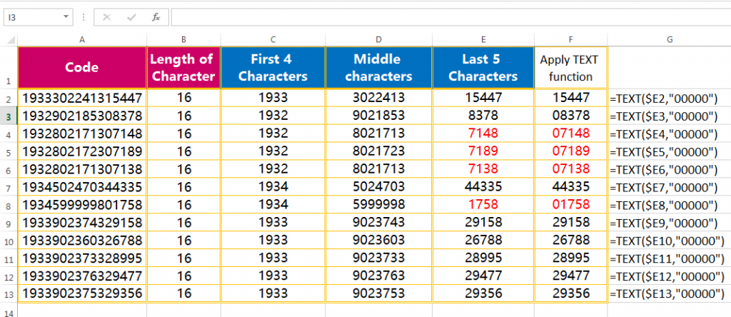
Text to Columns (Add zero value before any number by TEXT function)

• Convert Formulas into Values:

Either Copy (Ctrl+C) the selected range F1:F13 or the entire range A1:F13 and then select either the ‘Values and number formats’ (Alt+Ctrl+V+U or Alt+E+S+U) or ‘Values‘ (Alt+Ctrl+V+V or Alt+E+S+V) in the Paste Special dialog box.

■ Note: We had a detail discussed on Paste Special in Excel in a separate tutorial, suggested you read this tutorial: Paste Special in Excel Vs Break Link – Which one is Better?

[/su_box]

■ EXAMPLE 10: CONVERT NUMBERS WITH TRAILING MINUS SIGN TO NEGATIVE NUMBERS

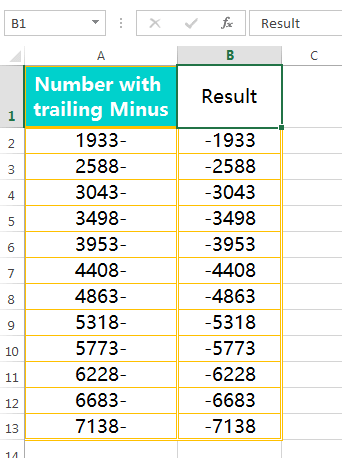
Sometimes we find a range of numbers with trailing minus signs and we want to make these numbers negative.

Text to Columns gives the perfect solution regarding this.

Here are the steps to convert this trailing minus into negative numbers:

• Select the data range (A2:A13) or the entire column (Column A)

• Press either Alt+D+E (sequentially press Alt, D, E) or Alt+A+E (sequentially press Alt, A, E) which will open the ‘Convert Text to Columns Wizard‘.

• In Step 1, select the Delimited (default option) radio button and then click Next or press Enter.

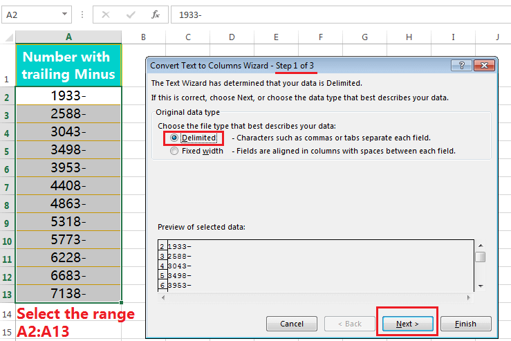
Text to Columns (Convert Numbers with Trailing Minus Sign to negative numbers)-1

• In Step 2, please notice that all the checkboxes should be unchecked if checked any. Then click Next or press Enter.

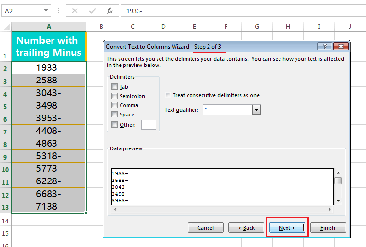
Text to Columns (Convert Numbers with Trailing Minus Sign to negative numbers)-2

• In Step 3, click on the Advanced button.

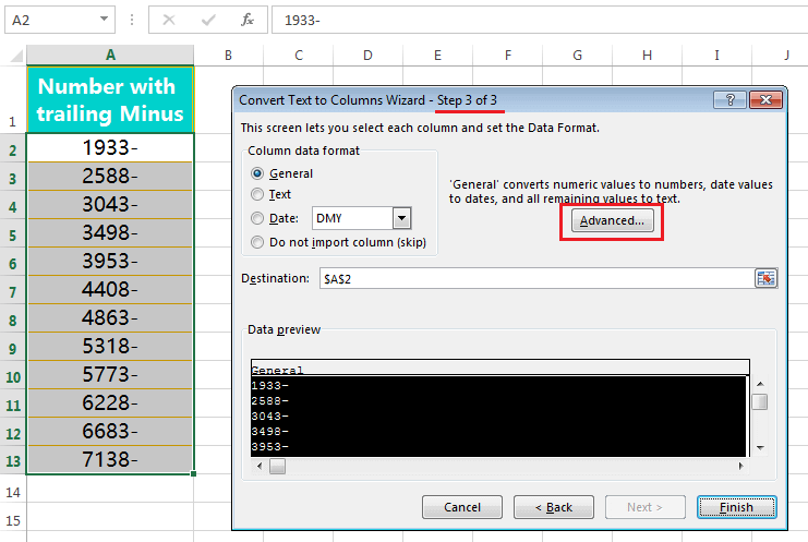
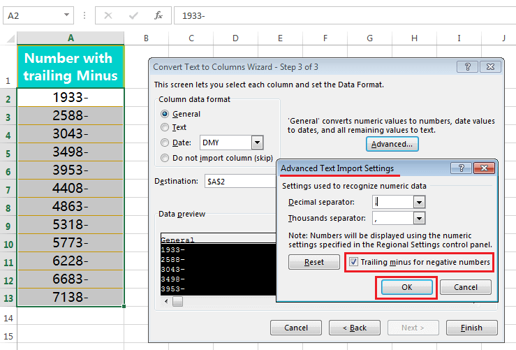
Text to Columns (Convert Numbers with Trailing Minus Sign to negative numbers)-3

In the Advanced Text Import Settings dialog box, select the ‘Trailing minus for negative number‘ option and then click OK or press Enter.

Text to Columns (Convert Numbers with Trailing Minus Sign to negative numbers)-4

• Select a new destination cell (i.e., B2) to avoid the overwriting of existing data.

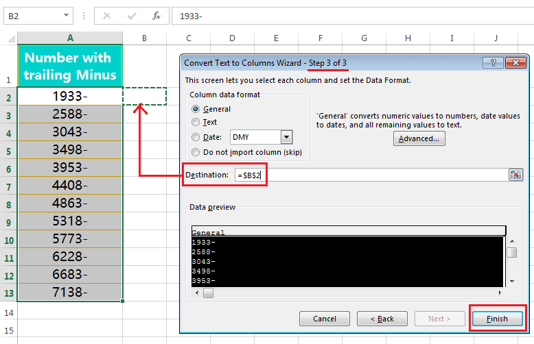
Text to Columns (Convert Numbers with Trailing Minus Sign to negative numbers)-5

• Click ‘Finish’ or press Enter. This would instantly place the minus sign from the end of the number to the beginning of it. Now we can easily use these numbers in formulas and calculations.

Text to Columns (Convert Numbers with Trailing Minus Sign to negative numbers)-6

(III). CONCLUSION

➢ Convert Text to Columns is basically used for the splitting of delimited text in Excel.

➢ Convert Text to Columns can work for a single column only at a time, it does not work with multiple columns.

➢ Other than the splitting of delimited text, it can also perform to convert ‘invalid date formats to a valid date format‘, convert ‘number to text‘ format and ‘text to number’ format.

➢ It’s another feature used in Excel to Convert Numbers with Trailing Minus Sign to negative numbers.

➢ It is also used to extract First/Last Few Characters of a fixed-width String in Excel.