09 Secrets: Must Know About Excel Tab and Scroll Bar?

(01). WHAT IS THE EXCEL TAB / TAB SHEET?

Excel tab Sheet is a visual label that looks like a file folder tab. In Excel, a sheet tab shows the of a worksheet contained in the workbook. 

Excel by default displays the Excel tab or tab sheet. Each Excel workbook contains at least one worksheet. We can create a number of worksheets in a workbook according to our requirements. Each worksheet shows as a tab at the bottom of the Excel window. These tabs help to manage the worksheets and move from one worksheet to another easily. 

(02). WHAT IS THE EXCEL SCROLL BAR?

Excel scroll bar is a navigation bar in a worksheet using to move to the right side and to move to the downward.

In addition to the sheet tab, Excel displays Vertical Scroll Bar to the right side and Horizontal Scroll Bar to the bottom of the Excel screen. These scroll bars help to scroll up-and-down and side-to-side through a worksheet, respectively. The arrow keys on the keyboard or the scroll wheel on the mouse helps to move the scroll bars.

(03). WHY EXCEL SCROLL BAR MISSING & EXCEL TABS NOT SHOWING?

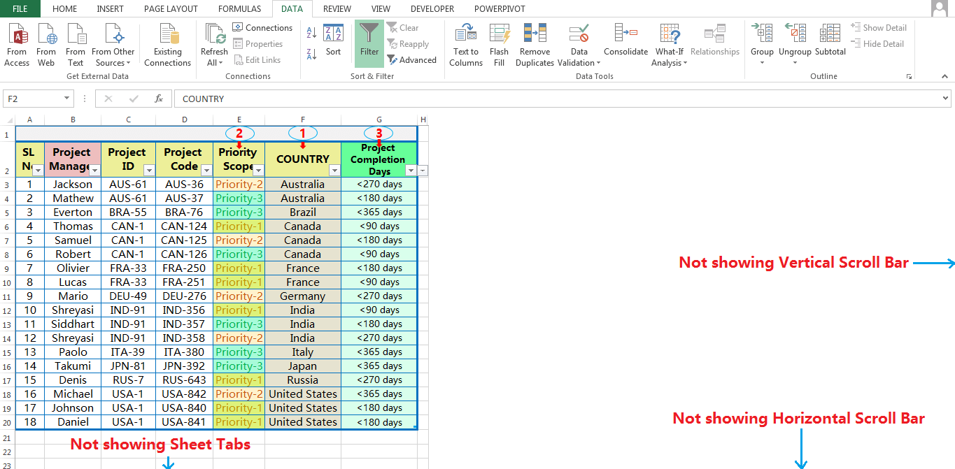
➢ Sometimes, while Excel opens it hides the scroll bar and sheet tab(s) accidentally.

➢ Sometimes, as per our requirement generally to increase the viewing area of the worksheet, hide the horizontal and vertical scroll bars manually.

Whatever is it, please note that changes in scroll bars and sheet tables are only applicable to the current workbook, not to other opened workbooks.

(i) Go to the File tab.

(ii) Select Options ➪ ‘Excel Options’ window opens.

Alternatively, use the excel shortcut Alt+F+T (sequentially press Alt, F, T) which will open the ‘Excel Options’ window.

(iii) Then select Advanced from the left sidebar ➪ scroll down to the Display options for this workbook section (about halfway down) ➪ select the Show horizontal scroll bar, Show vertical scroll bar, and Show sheet tabs checkboxes.

(iv) Click OK or press Enter to close the dialog box and return to the worksheet. 

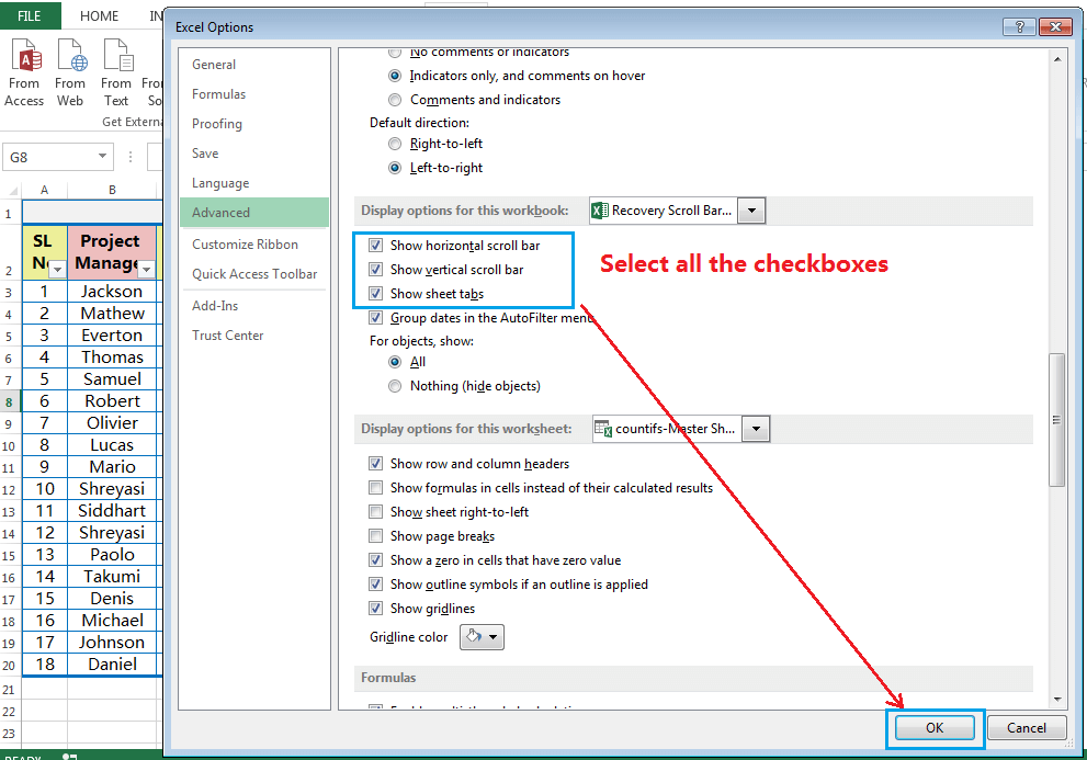
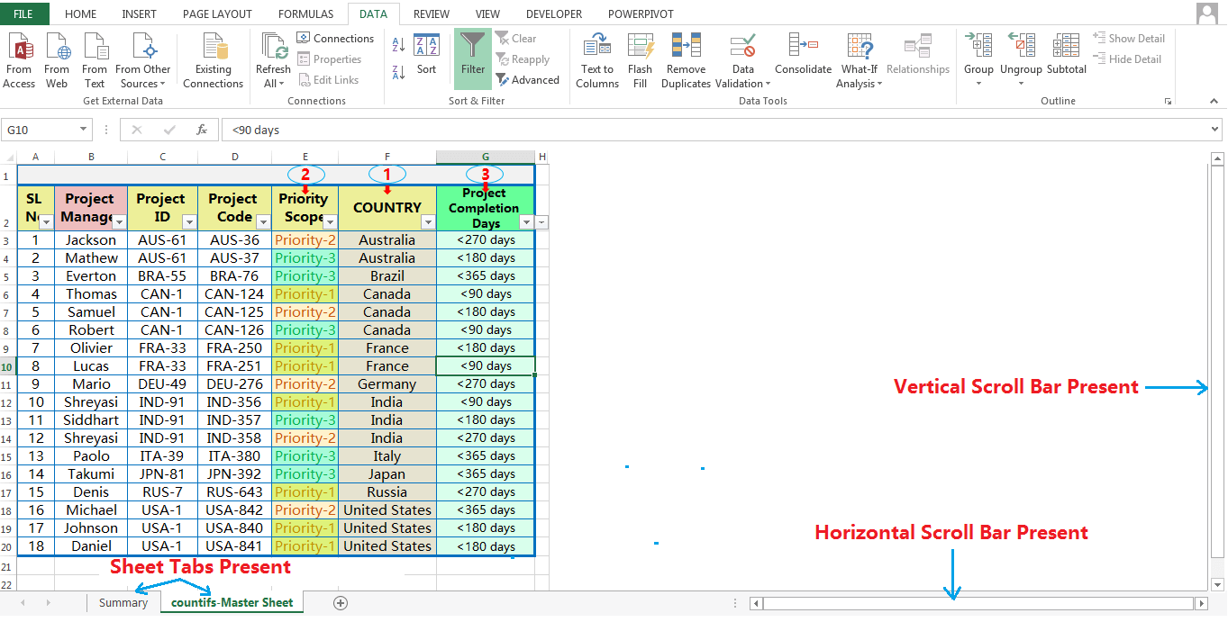
(v) The above process restores both the scroll bars and sheet tabs accordingly. If we uncheck all boxes, both the scroll bars and sheet tabs will hide. 

(04). HOW TO RESIZE THE HORIZONTAL SCROLL BAR IN EXCEL?

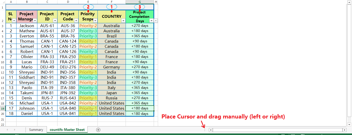
If there are a number of worksheets in a workbook, then the names of all tabs cannot be read at a glance. The only way to fix this is to shrink the size of the horizontal scroll bar manually.

Place the mouse pointer over the vertical ellipsis (three vertical dots) next to the horizontal scroll bar ➪ the mouse pointer changes to a double-headed arrow ➪ drag to the right to shrink the horizontal scroll bar or drag to the left to enlarge the scroll bar.

(05). HOW TO INSERT BLANK TAB SHEETS?

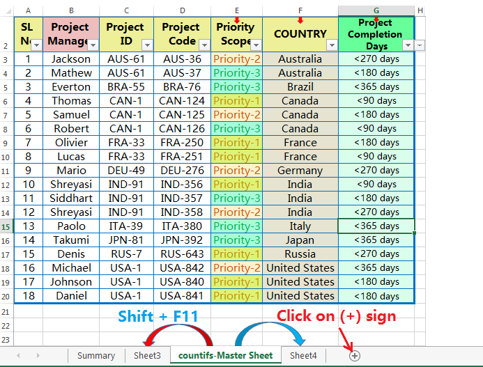
In a workbook, we can insert a Excel Tab or blank tab sheets in 3 ways: 

(A). Insert Blank Tab Sheets: Using the Plus (+) icon Right to the Tab Bar

To insert a new sheet tab / Excel tab in a workbook, click the tab after which we want to insert the worksheet ➪ then click the plus icon (+) to the right of the tab bar.

(B). Insert Blank Tab Sheets: Using the Excel Shortcut

Alternatively, the best way to insert a new sheet tab is to press Excel shortcut Shift+F11, a new worksheet is inserted before the selected tab.

 

Figure: Insert a tab by pressing right-click on the mouse

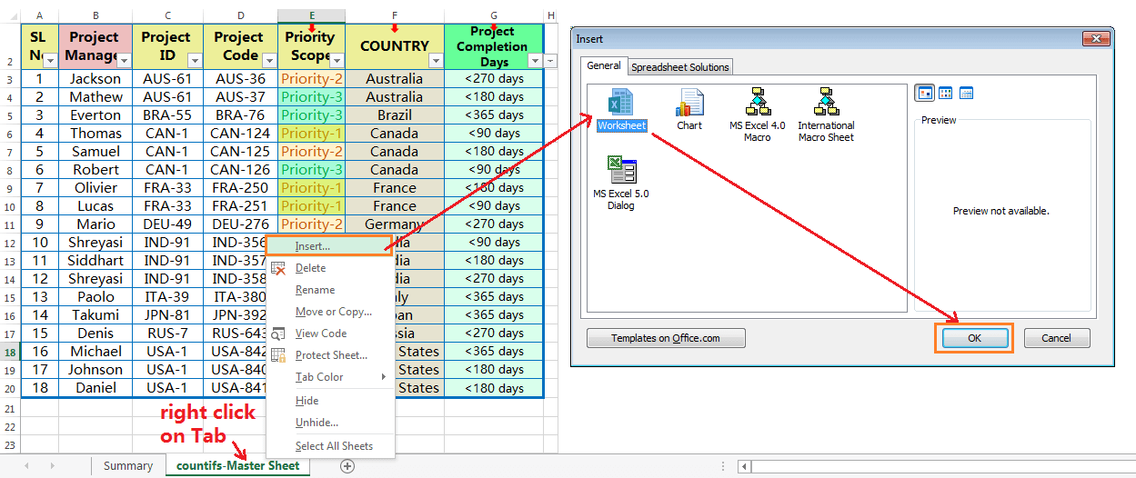
(C). Insert Blank Tab Sheets: Using the Ribbon

Alternatively, click the tab before which we want to insert the worksheet and then press right click on the mouse ➪ select Insert option ➪ Worksheet is selected by default ➪ Click OK or press Enter.

(06). HOW TO RENAME SHEET IN EXCEL?

Each workbook comprises one or more worksheets, and each worksheet is made up of individual cells. Each cell contains a value, a formula, or text. A worksheet also has an invisible draw layer, which holds charts, images, and diagrams. Each worksheet in a workbook is accessible by clicking on the tab sheet at the bottom of the workbook window.

By default, new tabs are named as Sheet1, Sheet2, etc., in sequential order. That means if there are multiple worksheets in a workbook, and each sheet has its name displayed in a sheet tab. It is helpful to rename each tab according to the database subject (max 31 characters long) to help us organize and find the data easily.

There are 03 ways to rename the Excel tab. Remember that each tab must have a unique name.

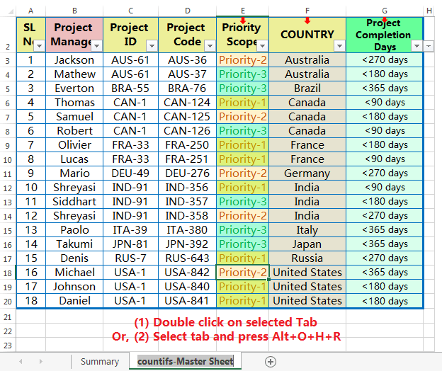
(A). Rename Sheet in Excel: Using the Mouse Double Click

Simply double click on the tab want to rename ➪ type a new name and press Enter.

(B). Rename Sheet in Excel: Using the Excel Shortcut

Press Excel Shortcut Alt+O+H+R (sequentially press Alt, O, H, R) which will activate the sheet rename ➪ type a new name, and press Enter.

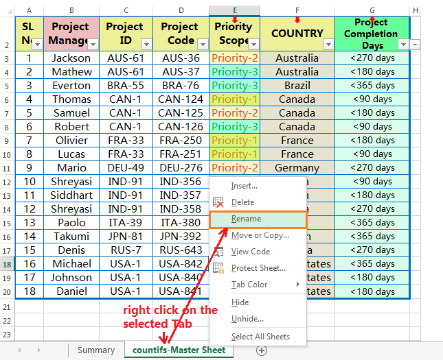
(C). Rename Sheet in Excel: Using the Mouse Right Click

Right-click on the selected Tab and click on the ‘Rename’ option ➪ type a new name and press Enter.

(07). MOVE OR COPY THE EXCEL TAB

If we can make an exact copy of the Excel tab (worksheet), we should try to avoid copy-paste to another new worksheet rather we prefer to use Move or Copy Tab to another location in the same workbook or another open workbook.

We can move or copy the Excel tab in two ways:

(A). Move or Copy the Excel Tab: Using Mouse Right Click

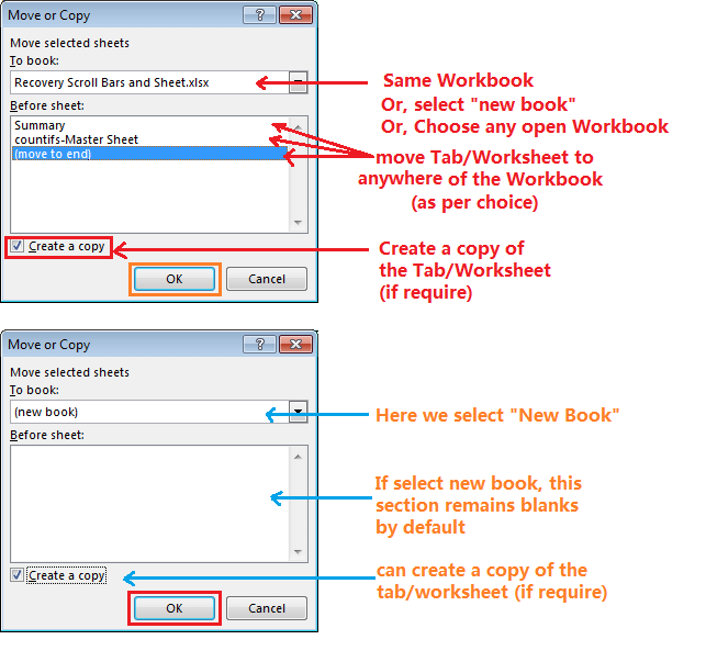
(i) Right-click on the sheet tab(s) want to move or copy ➪ select Move or Copy ➪ Open the Move or Copy dialog box, the currently active workbook is selected by default in the To Book drop-down list.

If we want to copy or move the tab to another existing workbook, make sure that this workbook should be opened and select it from the list. But if we want to copy or move the tab to another new workbook, just select the (new book) option from the list.

(ii) Then we move to the Before sheet list box just below the To Book, select the worksheet (tab) before which we want to insert the copied (or moved) tab.

(iii) After that, we go to the third option Create a copy. If we want to copy the tab, but not moving it, make sure the Create a copy box is checked and click OK. As a result, the duplicate tab is created. If the Create a copy box is not checked, the tab will be moved to the chosen location instead of copied.

(iv) Click on OK or press Enter to apply the activity.

(B). Move or Copy the Excel Tab: Using the Excel Shortcut

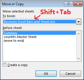
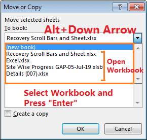
(i) Similarly, we can move or copy the Excel tab by using an Excel shortcut: Select the tab(s) want to move or copy ➪ press Alt+E+M  (sequentially press Alt, E, M) to open the Move or Copy dialog box ➪ then press Shift+Tab which helps to go to the To Book drop-down list. Press Alt+Down Arrow (⬇) which will open the drop-down list. Select either (new book) or any one of the opened workbooks we want to copy or move the tab. Press Enter or click OK.

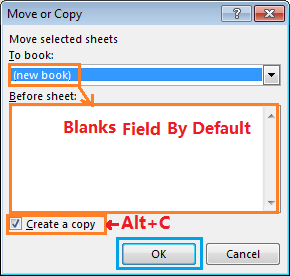
(ii) Then press Tab to move to the ‘Before sheet:’ list box section and choose the worksheet (tab) by up or down arrow keys before which we want to insert the copied (or moved) tab. Remember that if we select the (new book) option, then the Before sheet section remains blank.

(iii) In the third step, press Alt+C which will select the Create a copy checkbox.

(iv) At last, click OK by pressing the Spacebar or press Enter to apply the activity.

 

 

(08). HOW TO DELETE THE EXCEL TAB?

We can delete the unnecessary tab(s) from a workbook in two ways:

(A). Delete the Excel Tab: Using the Mouse Right Click

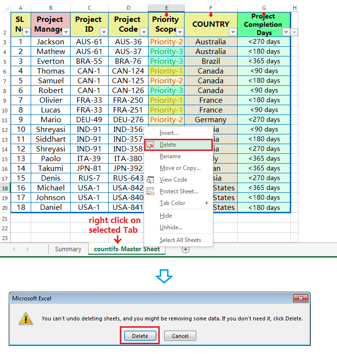
Right-click on a tab or on the multiple tabs (select by pressing Ctrl key) want to delete ➪ Select Delete from the list ➪ Excel window appears for getting confirmation from the user to delete it permanently, click on the Delete or press Enter. A worksheet or Tab has removed from the workbook.

(B). Delete the Excel Tab: Using Excel Shortcut

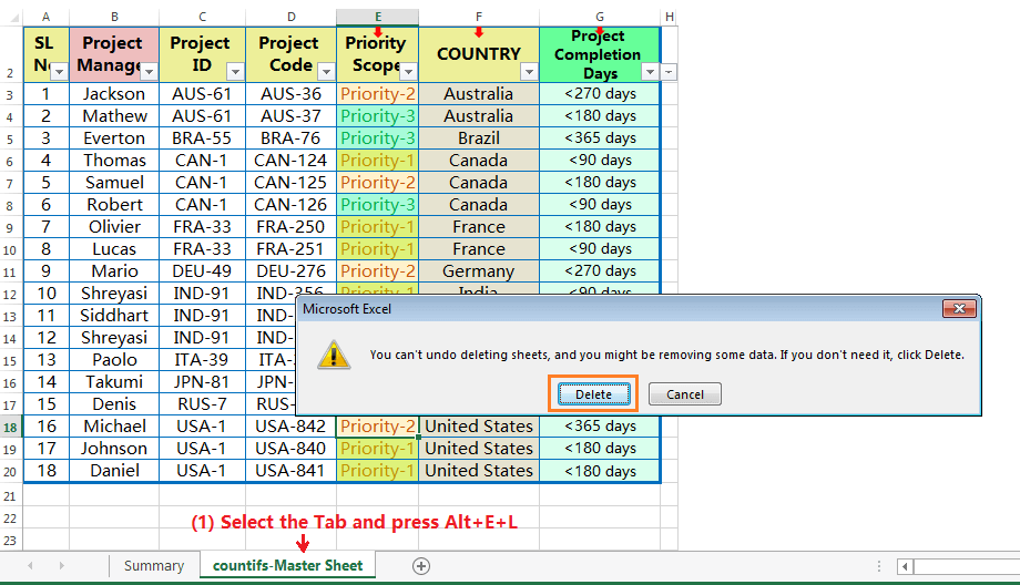
Simply select the tab or tabs by pressing the Ctrl key we want to delete ➪ then press Alt+E+L (sequentially press Alt, E, L) ➪ an Excel window appears for getting confirmation from the user to delete it permanently, either click on Delete or press Enter. The selected worksheet or Tab has been removed from the workbook permanently.

(09). HOW TO HIDE OR UNHIDE TABS IN EXCEL?

Microsoft Excel shows sheet tab(s) at the bottom of the worksheet by default, which helps to navigate from one worksheet to another worksheet easily. 

Most of the time, Excel users make different types of dashboards, kinds of summaries, and apply a combination of formulas in different worksheets based on the master database, but they would rather not show that data to other users. In this situation, they prefer to hide the worksheet(s). Remember that Excel allows hiding all worksheets except at least one. 

We can hide the tab(s) from a workbook in three ways: 

(A). Hide the Excel Tab(s): Using the Mouse Right Click

Select one or multiple worksheet tabs we want to hide in the Tab bar. 

How to Select Multiple Excel Tabs or Worksheets?

⇒ If we want to select multiple adjacent tabs, click on the first tab and hold the Shift key and then click on the last tab. Therefore, multiple adjacent tabs or contiguous tabs are selected at a glance. 

⇒ If we want to select multiple non-adjacent tabs or non-contiguous tabs, then click on the individual tab one by one holding the Ctrl key. 

After selecting the Tab or multiple tabs,  right-click on the selection and select Hide from the context menu. Thus the selected tabs will be hidden from the Tab bar. 

(B). Hide the Excel Tab(s): Using the Excel Shortcut

Select the contiguous tabs with the Shift key or non-contiguous tabs with the Ctrl key ➪ then press Alt+H+O+U+S (sequentially press Alt, H, O, U, S) Thus, all tabs would be hidden in a moment.

(C). Hide the Excel Tab(s): Using the Ribbon

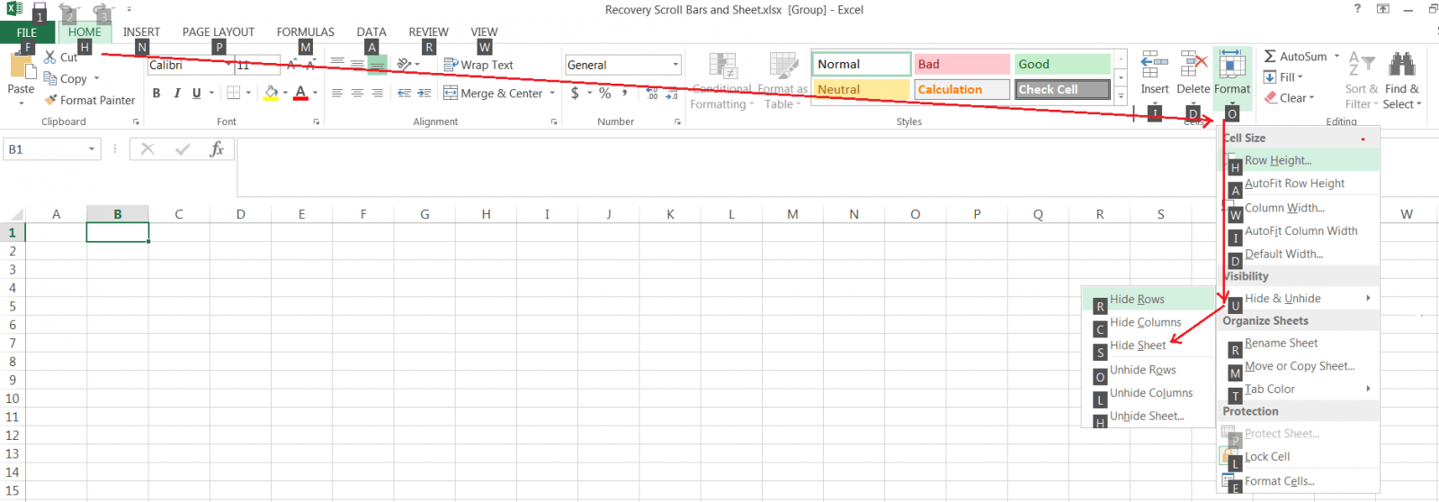
Select the contiguous tabs with the Shift key or non-contiguous tabs with the Ctrl key ➪ Go to the Home tab ➪ Click on the Format drop-down in the ‘Cells‘ group ➪ Under Visibility section, point to the Hide & Unhide, a list opens and select the Hide Sheet. 

(10). HOW CAN PERFORM EXCEL TAB NAVIGATION?

If there are multiple tabs, they may not all display at once, depending on the size of the Excel window. There are a couple of ways we can navigate from one tab to another.

(A). Excel Tab Navigation: Using Three Horizontal Dots

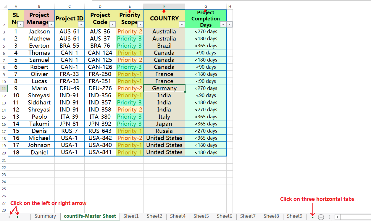
There are three horizontal dots on one or both ends of the tab bar. If we click on the three dots on the left end, we navigate to the first tab in the left direction. If we click on the three dots on the right end, we navigate to the last tab in the right direction.

(B). Excel Tab Navigation: Using Right or Left Arrows

We can also click the right or left arrows on the left side of the tab bar to scroll through the tabs.

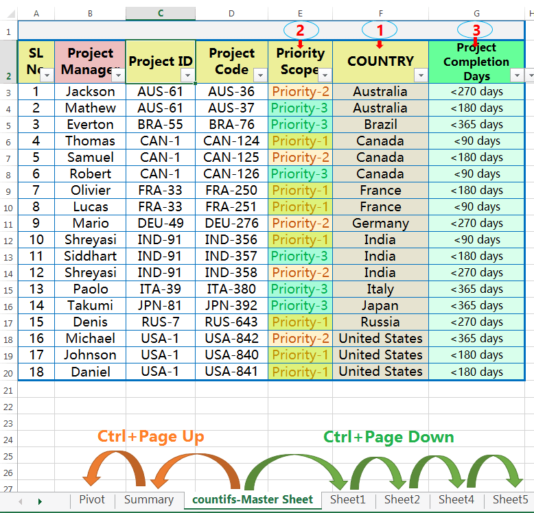
(C). Excel Tab Navigation: Using Excel Shortcut

The best way to move from one tab to the adjacent tab by using the Excel shortcut.

➢ Ctrl+Page Down: Navigate towards the right side 

➢ Ctrl + Page Up: Navigate towards the left side 

(11). HOW TO CHANGE TAB COLOR IN EXCEL?

If there are multiple tabs in a workbook, then tab identification, tab navigation becomes difficult. Thus we would like to use the same tab color with similar activity and make a group. For example, all types of ‘Summary tabs’ in a workbook to make a group with the same type of color.  Similarly, all pivot table tabs to make a group with the same tab color. Therefore, we can easily identify the tabs by tab colors.

We can color the tab(s) in 03 ways: 

(A). Change Tab Color in Excel: Using the Mouse Right Click

Select one or multiple worksheet tabs we want to make a group with a similar color ➪ right click on the selection with mouse ➪ go to the Tab Color ➪ a right-side color palette window opens ➪ choose any color and click on it.

(B). Change Tab Color in Excel: Using the Excel Shortcut

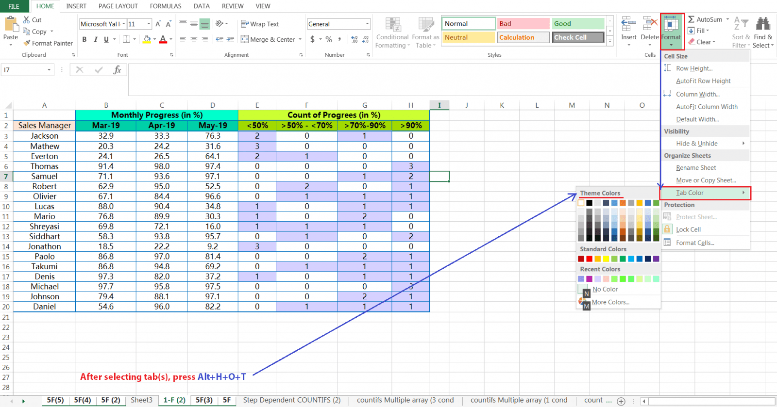
Select one or multiple worksheet tabs we want to make a group with similar color ➪ then press Alt+H+O+T (press sequentially Alt, H, O, T) ➪ choose any color from the color palette, and click on it.

(C). Change Tab Color in Excel: Using the Ribbon

Select one or multiple worksheet tabs we want to make a group with similar color ➪ go to the ‘Home’ tab ➪ then click on the ‘Format’ drop-down under Cells section ➪ place the cursor on Tab Color ➪ a  right-side color palette window opens ➪ select any color from the palette and click on it.