04 Best Methods: How To Merge Cells in Excel?

What is Merge Cells in Excel? How to Merge Cells in Excel? – Both questions are valid in every Excel users’ mind. In this tutorial, we explain 03 different methods to apply Merge Cells and Unmerge Cells in Excel as well.

The Merge & Center in Excel is a useful feature that combines (or merges) the selected cells row-wise or column-wise and merges them into a single cell. As a result, merge the values of two or more columns (or multiple rows) into a single column (or single row).

Merge cells never combine the contents of cells. Rather, it combines a group of cells into a single cell that occupies the same space.

We can merge any number of cells occupying any number of rows and columns. Similarly, in the same way, we can unmerge them also.

It is typically used for row and column headings in tables of data, where we would like one title to apply to many cells.

The range that intends to merge should be empty, except for the upper-left cell. If any of the other cells that intend to merge are not empty, Excel displays a warning. If we continue, all the data (except in the upper-left cell) will be deleted. To avoid deleting data, click Cancel in response to the warning.

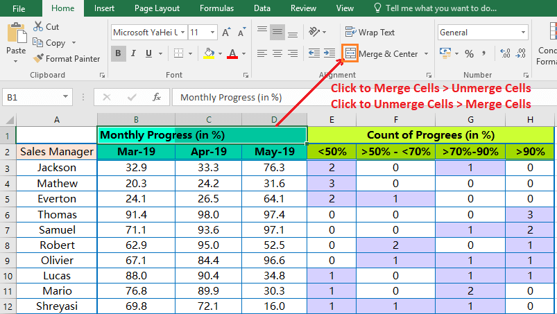
To merge cells, select the cells that we want to merge and then click the Merge & Center” button. The cells will be merged, and the content in the upper-left cells will be centered horizontally. The Merge & Center button acts as a toggle.

Similarly, in the case of unmerging cells, select the merged cells, and click the Merge & Center button again.

(I). HOW TO MERGE CELLS IN EXCEL SHORTCUT

On the Home tab, “Merge & Center” contains a drop-down list with four options. We can avail of these options with the Excel shortcuts mentioned below:

Table: Merge Options and Excel Shortcut

[su_table]

Option	Excel Shortcut	Results
Merge and Center	Alt+H+M+C (sequentially press Alt, H, M, C)	Merge the selected cells and center the text across the merged cells.
Merge Across	Alt+H+M+A (press sequentially Alt, H, M, A)	Merges the selected cells, but keeps the text left-aligned or values right-aligned.
Merge Cells	Alt+H+M+M (press sequentially Alt, H, M, M)	Merges a range of cells on multiple rows as well as in multiple columns.
Unmerge Cells	Alt+H+M+U (press sequentially Alt, H, M, U)	Separates a merged cell into multiple cells again.

[/su_table]

■ Note: We had detail discussed on Excel shortcuts in separate two tutorials, suggested you read these tutorials:

80+ Excel Shortcuts with ALT Key || Best Hotkey of Keyboard Shortcuts

90+ Best Excel CTRL Shortcuts | Useful Keyboard Shortcuts |

(II). HOW TO MERGE CELLS IN EXCEL?

We can join multiple cells to make one larger cell by using one of the three different options for merging cells.

• Merge & Center
• Merge Across
• Merge Cells

Only the data in the far left cell (or top-right cell) are merged. Any other data in the merged cells are deleted. Excel merges the selected cells together into one cell, and the merged cell address is that of the original cell on the left.

STEPS TO START:

• Step 1: Enter the text in the top-left cell of the range.

• Step 2: Select the range of cells across which we want to center the label.

• Step 3: We can select Merge and Center options any of the following 03 Methods:

■ METHOD 1: HOW TO MERGE CELLS IN EXCEL SHORTCUT

To apply the Merge Cells (usually used Merge and Center option), use the Excel shortcut Alt+H+M+C (sequentially press Alt, H, M, C).

■ METHOD 2: HOW TO MERGE CELLS IN EXCEL ➢ USING THE ‘MERGE & CENTER’ CONTROL BUTTON 

Go to the Home tab ➪ Alignment section ➪ Click on the ‘Merge & Centre’ control button which will merge the cells, and the content in the upper-left cells will be centered horizontally. The Merge & Center button acts as a toggle.

■ METHOD 3: HOW TO MERGE CELLS IN EXCEL ➢ USING THE ‘MERGE & CENTER’ DROP-DOWN

Alternatively, go to the Home tab ➪ Alignment section ➪ Click on the ‘Merge & Centre’ drop-down and select the Merge & Center option from the drop-down list.

■ METHOD 4: HOW TO MERGE CELLS IN EXCEL ➢ USING THE ‘FORMAT CELLS’ DIALOG BOX

Press Ctrl+1 which will open the ‘Format Cells’ dialog box ➪ Go to the ‘Alignment’ tab ➪ Choose ‘Center’ from the Vertical drop-down list ➪ Then select the Merge cells checkbox under the Text Control section ➪ Either press Enter or click OK to apply the condition.

(III). HOW TO UNMERGE CELLS IN EXCEL?

Similarly, if we want to split a merged cell into multiple cells, then follow any of the below methods. However, after unmerging the data places in the top-left cell.

■ METHOD 1: HOW TO UNMERGE CELLS IN EXCEL SHORTCUT

In the case of unmerging cells, select the merged cells ➪ Then press Excel shortcut Alt+H+M+C (sequentially press Alt, H, M, C).

■ METHOD 2: HOW TO UNMERGE CELLS IN EXCEL ➢ USING THE ‘MERGE & CENTER’ CONTROL BUTTON

Select the merged cells ➪ Go to the Home tab ➪ Alignment section ➪ Click on the ‘Merge & Centre’ control button which will unmerge the cells.

■ METHOD 3: HOW TO UNMERGE CELLS IN EXCEL ➢ USING THE ‘MERGE & CENTER’ DROP-DOWN

Alternatively, Select the merged cells ➪ Go to the Home tab ➪ Alignment section ➪ Click on the ‘Merge & Centre’ drop-down and select the Unmerge Cells option from the drop-down list.

■ METHOD 4: HOW TO UNMERGE CELLS IN EXCEL ➢ USING THE ‘FORMAT CELLS’ DIALOG BOX

Select the merged cells ➪ Press Ctrl+1 which will open the ‘Format Cells’ dialog box ➪ Go to the ‘Alignment’ tab ➪ Choose ‘Center’ from the Vertical drop-down list ➪ Then deselect the Merge cells checkbox under the Text Control section ➪ Either press Enter or click OK to apply the condition.

All the above methods split all the merged cells, but only the upper-left cells will be filled with data. Rest cells are kept blank.

(IV). HOW TO UNMERGE CELLS IN EXCEL WORKSHEET?

If we want to unmerge all the cells in the worksheet, then we select the entire worksheet by pressing Ctrl+A (hold the Ctrl key and press the A key twice) or click on the Select All icon (a little inverted triangle is located at the left corner of the worksheet).

After selection of the entire worksheet, if we find that the Merge & Center button is highlighted which indicates the presence of merge cells in the worksheet.

To unmerge cells in Excel worksheet, we can either

(i) Press Alt+H+M+C (sequentially press Alt, H, M, C);

(ii) Click on the highlighted Merge & Center button (toggle);

(iii) Click on the Merge & Center drop-down ➪ select Unmerge Cells from the drop-down list.

(iv) Press Ctrl+1 which will open the Format Cells dialog box ➪ Alignment tab ➪ Uncheck the Merge cell checkbox under Text control ➪ Click OK or press Enter.

■ Note: If the Merge & Center button is not highlighted which indicates there are no merge cells in the worksheet.

(V). LIMITATIONS OF MERGE CELLS IN EXCEL

In Excel, generally, we apply to merge cells when the same values of multiple cells to be merged into one, or we may need to present the data differently.

Now the question arises in mind, why do we find the merged cells in our worksheet or database?

Because Merge cells create big limitations in Excel and we should know about those step by step:

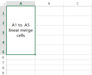
(01) Merge cells generally form either a linear shape or a rectangular shape.

For example, we can merge cells in linear shape like A1, A2,….A5 or A1, B1, C1,….E1

Linear shaped merge cells

Rectangular shaped Merge Cells

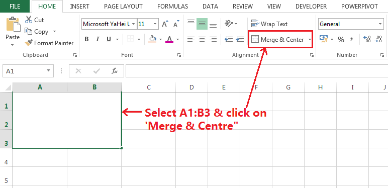
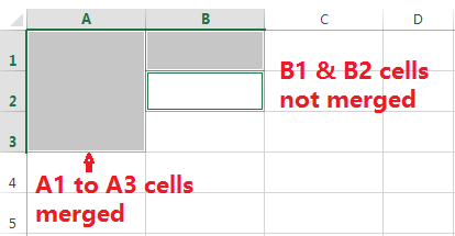
We can merge cells in rectangular shape likes, A1, A2, A3, and B1, B2, B3; but we cannot merge just cells A1, A2, A3, and B1, B2. In this case, only the first linear cells are merged, i.e. A1 to A3 but not B1 & B2.

(02) In Excel, merge cells only merge the two or more cells, but can’t merge the contents.

If only one of the original cells contains data, the merged cell will keep this data.

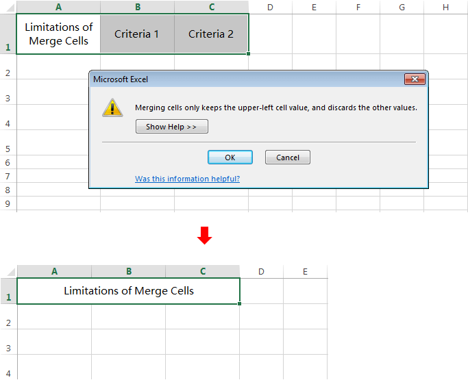
However, if more than one of the original cells contains data, the merged cell will only keep the data from one of the original cells (generally the left upper cell in the range). Additionally, a warning message appears about this, before Excel completes the merge.

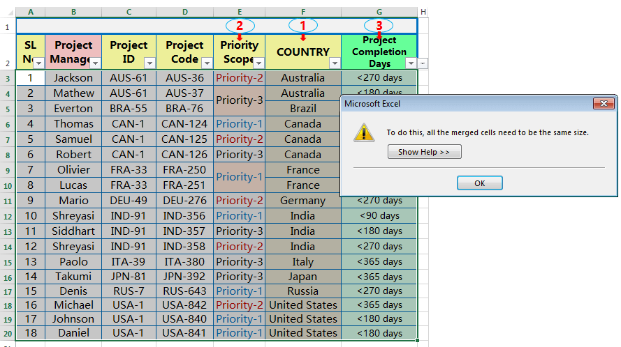
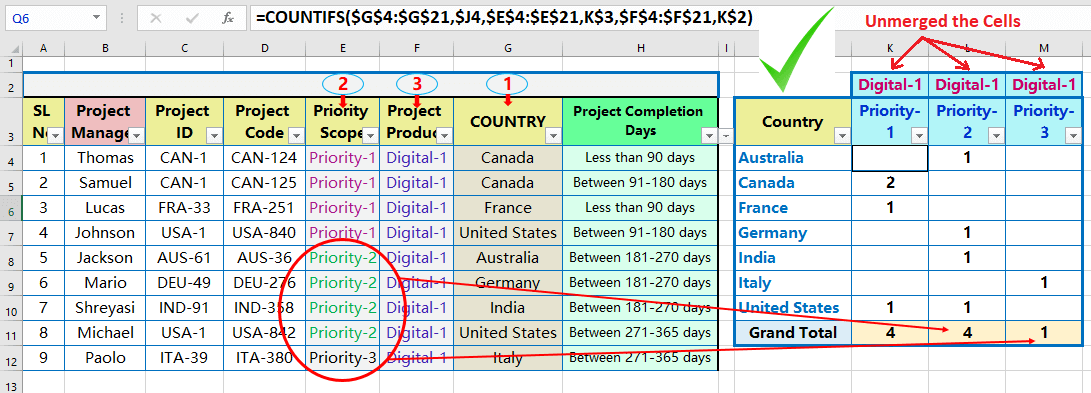
For example, in the given table, we find that the “Priority scope” column has merged cells; but if we managed to sort another column in the same table/dataset likes “Project Completion Days” will give a warning message, though it has no merged cell at all.

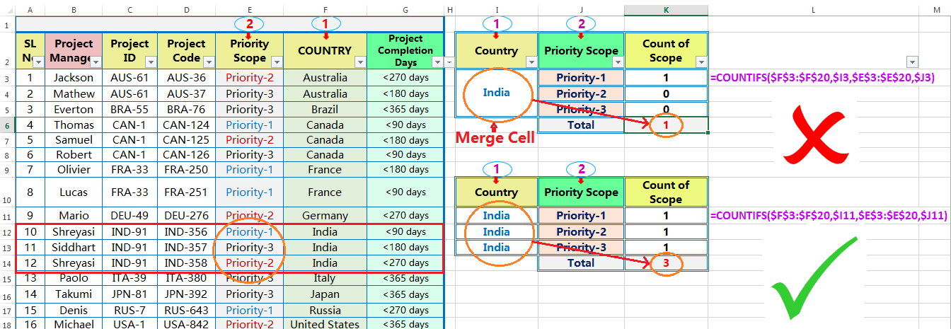
(04) Once criteria cells are merged inside a table, any excel formula only captures the value of the left upper cells, the rest merged cells considered as blanks.

For example, in the first instance, especially for merging cells, the COUNTIFS functions count the scope of India 1 instead of 3.

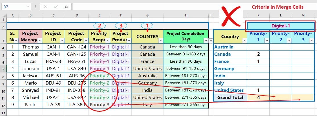
(05) Similarly, if the criteria cells are merged in a table heading, COUNTIFS (Conditional Count) or SUMIFS (conditional Sum) formula returns an erroneous/inappropriate result. In that case, Excel only considers the first upper left cell value in the formula.

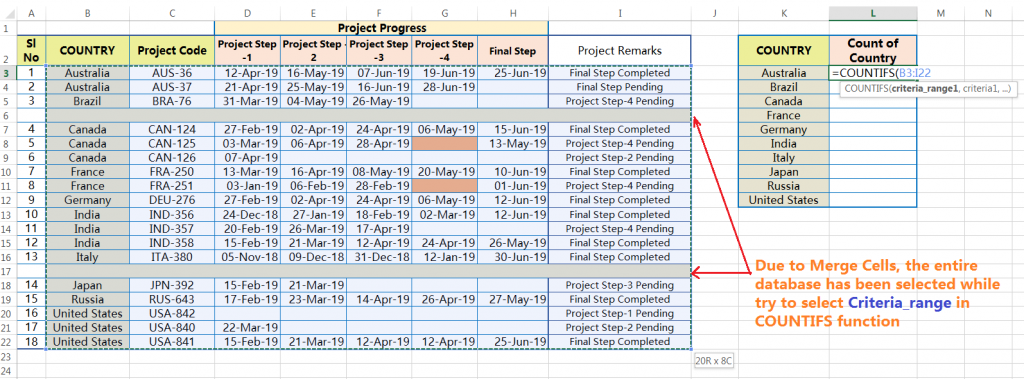
(06) If cells are merged into the main database, it is difficult to select a single column range.

Excel formulas like VLOOKUP(), HLOOKUP(), COUNTIFS(), SUMIFS(), INDEX(), and MATCH(), etc., considered the entire range as an array range until the end of the merge cells. So in this scenario, formulas cannot be worked dynamically. So we manually count the column number (for the col_index_num) for VLOOKUP.

(07) If we try to paste a larger database over a smaller database, Excel easily overlaps the smaller database.

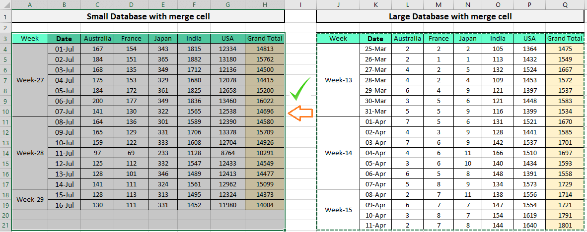
But if we try to paste a smaller database (having merged cells) into a larger database (also having merged cells), Excel will not allow pasting over it.

(VI). ALTERNATIVE OF MERGE CELLS IN EXCEL?

Without applying the Merge and Center option, we can center the content across the selected range without merging cells. So we can get rid of the limitations of merge cells in Excel.

Select the range of cells that we want to merge and center the content ➪ Press Ctrl+1 which will open the Format Cells dialog box ➪ Go the Alignment tab ➪ Click on the Horizontal drop-down and select Center Across Selection ➪ Click OK.

As a result, this would center the content across the selection without merging cells and we can select each cell individually. We can easily insert a column with the Ctrl+Spacebar.  We can easily avoid the error while sorting a data.

(VII). HOW TO FIND MERGE CELLS IN EXCEL?

So the next question arises in our mind, how do we find merged cells in our worksheet? As merging cells relate to alignment, and alignment is part of the formatting, thus Excel can find the merge cells by format.

➢ STEP 01: OPEN THE FIND DIALOG BOX

We can find merge cells in Excel with the Find dialog box. However, we can open the Find dialog box either in two ways:

Method 1: Using the Excel Shortcut

Place cursor anywhere in the worksheet ➪ Then press Ctrl+F which will open the ‘Find‘ tab in the ‘Find and Replace’ dialog box.

■ Note: We had detail discussed on Find and Replace in a separate tutorial, suggested you read this tutorial: 07 Points Guided You How to Find And Replace in Excel?

Method 2: Using the Ribbon 

Go to the Home tab ➪ Click on the ‘Find & Select’ drop-down in the Editing section ➪ Select the Find option which will open the ‘Find’ tab under the ‘Find and Replace’ dialog box.

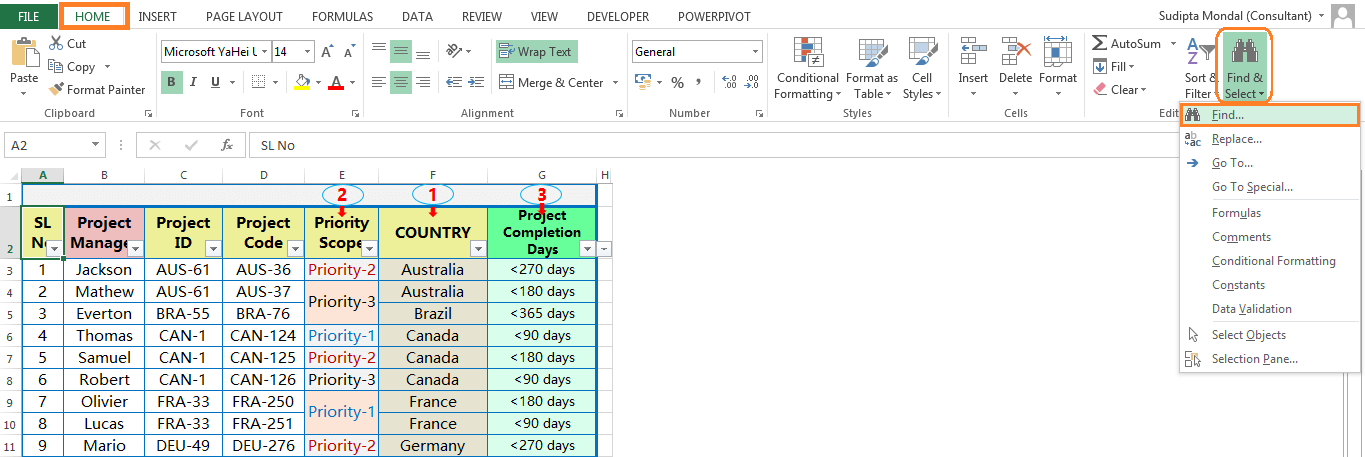
➢ STEP 02: SWITCH TO THE ‘ALIGNMENT’ TAB

In the Find dialog box, click on the ‘Options‘ button which will open the Advanced option ➪ Then click on the ‘Format…’ box which will open the Find Format dialog box ➪ Switch to the ‘Alignment’ tab.

➢ STEP 03: SELECT THE ‘MERGE CELLS’ CHECKBOX

In the Alignment tab, select the Merge cells checkbox under the Text control section ➪ Finally, click OK or press Enter.

➢ STEP 04: RETURN TO THE ‘FIND AND REPLACE’ DIALOG BOX

We return to the Find tab under the ‘Find and Replace‘ dialog box again and click either on the:

⇒ Find Next to get to the next merged cell.

⇒ Find All to get a list of all merged cells.

When we click on one of the list items, Excel will trace the corresponding merged cell in the worksheet:

Note: If there are any merged cells in a specific range (either in a column or a row range), select that range and cast a glance at the ‘Merge & Center’ button. If we found that the button is highlighted which indicates that there is at least one merged cell in the selected range.

(VIII). HOW TO COPY THE ORIGINAL VALUE FROM ABOVE UNMERGE CELLS IN EXCEL?

After unmerging, a number of blank cells leftover in the dataset. So in this case, we can fill them with the values from above unmerged cells.

Select the dataset with Ctrl+A ➪ Press Ctrl+G or F5 which will open the Go To dialog box.

Then click on the Special button or press Alt+S (hold down the Alt key and then press S) which will open the Go To Special dialog box ➪ Either select the Blanks radio button or press Alt+K (hold down the Alt key and press K) ➪ Click OK or press Enter.

As a result, all the blanks are selected at a glance.

■ Note: We had detail discussed on Go To Special in a separate tutorial, suggested you read this tutorial: 12 Examples || How to Use Excel Go To Special?

After selecting the blank cells, type and equality sign (=) and press the Up Arrow (⬆) key on the keyboard. As a result, this will create a simple formula and fill the cell with the value from above unmerged cell.

To apply the formula in all the blank cells simply press Ctrl+Enter (hold down the Ctrl key and then press the Enter key).

As a result, all blank cells are filled with the values of the above cells.

• All the Formulas to be Converted into Values:

Then select the dataset with Ctrl+A ➪ Copy (Ctrl+C) ➪ Press Alt+E+S+V (sequentially press Alt, E, S, V) or press Alt+Ctrl+V+V (hold down Alt+Ctrl+V, then press V) which will select the ‘Values‘ option in the Paste Special dialog box ➪ Either press Enter or click OK.

As a result, all the formulas in the dataset are converted into values.