Understanding Excel Operators – Guide

“Operator! How can I help you?”

This is what you hear when you call an operator in a hotel or company etc. Operators are there to help. Their operation is to implement and execute your command.

Even a simpler example is to ask someone “what is 2+2?” With this question you are also giving away what to do with two 2s. You asked to ADD them. Hence the other person will perform the operation of adding and give you the result “4”

Same way Excel is there to help you. You give it a task and also tell it how to operate. For example to ask Excel to do the same you have to write a formula =2+2 and press Enter. Excel will return 4. Again it is the “+” sign that completed the command. Hence the name operator.

In Excel we have several operators that we must know especially while writing formulas. Following is the list of operators I know so far with their names, what they do and some examples for each:

[table id=1 /]

1 Arithmetic operators

1.1 Basic arithmetic operators: + – * /

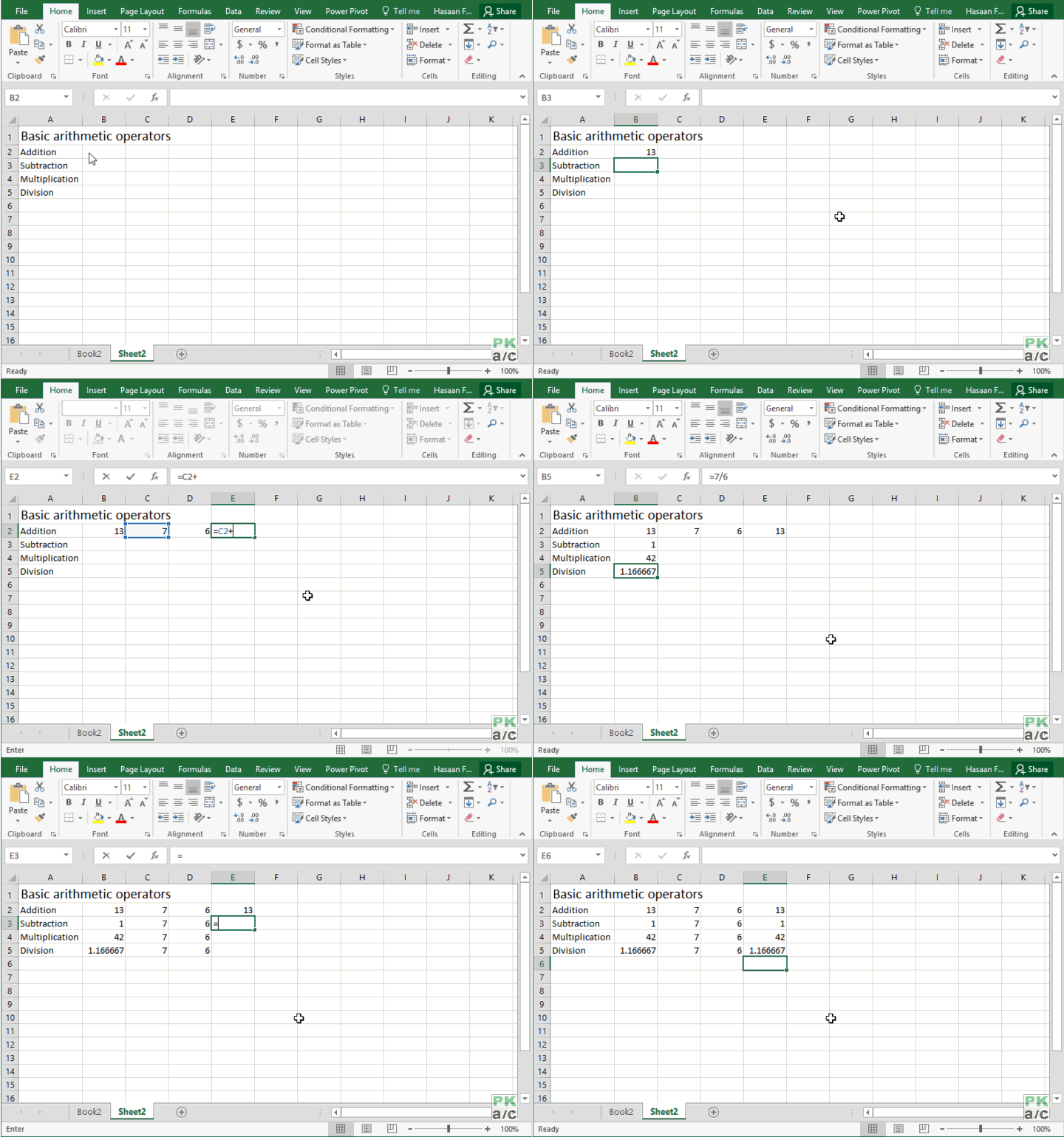
Addition, Subtraction, Multiplication and Division are done in almost same fashion as we normally do in real life. The only difference is that instead of using X for multiply we use asterisk *.

1.2 Exponent, Percentage and Parenthesis

Exponent and percentage operators are again simple. The role of parenthesis is same as we learnt in 4th grade mathematics

2 Reference operators

2.1 Range operator

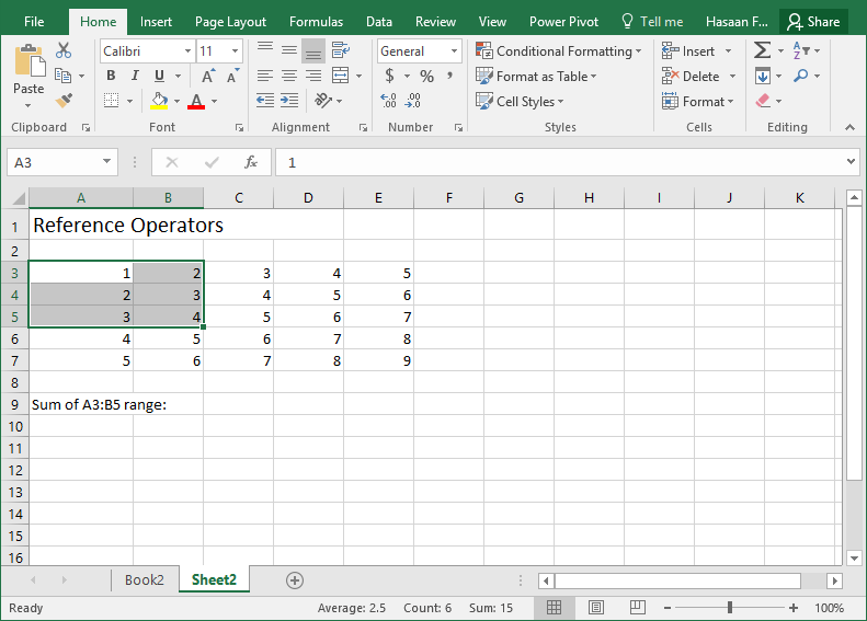
In excel we use colon (:) to specify range. In the following figure range A3:B5 include cells A3, A4, A5 and B3, B4, B5. As you can see the range is starting from the cell mentioned on the left of colon and ending on the cell mentioned on the right of colon.

To sum the values in range A3: B5 we will the formula: =SUM(A3:B5)

2.2 Range union operator

To combine two ranges of data inside formula we use comma (,). For example if I have to combine range A3:B5 and C6:E7 then I will write it liks this: (A3:B5,C6:E7). Following figure shows the ranges shaded in gray:

To find the sum of unified ranges the formula will be: =SUM(A3:B5,C6:E7)

2.3 Range intersection operator

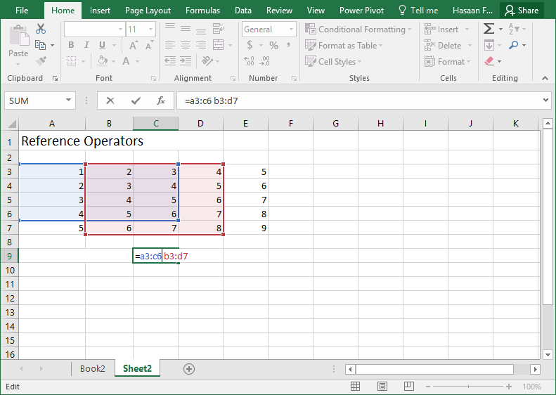
Intersection operator determines the range that is common between two specified ranges and is denoted with a (space). For example the intersection of ranges A3:C6 and B3:D7 is B3:C6 as it is common in both ranges. As you can observe intersecting range starts from the first cell of subsequent range i.e. B3 and ends at the last cell of former mentioned range i.e. C6

Following figure shows the intersecting range enclosed in both blue and red boxes:

In order to sum value of intersecting range within A3:C6 and B3:D7 the formula will be: =SUM(A3:C6 B3:D7)

2.4 Absolute reference operator

This operator works on cell references and comes handy when you use quick fill meaning when you drag the fill handle up, down, right or left. Remember cell reference is a combination of row and column address. For example cell B3 is in column B and row 3.

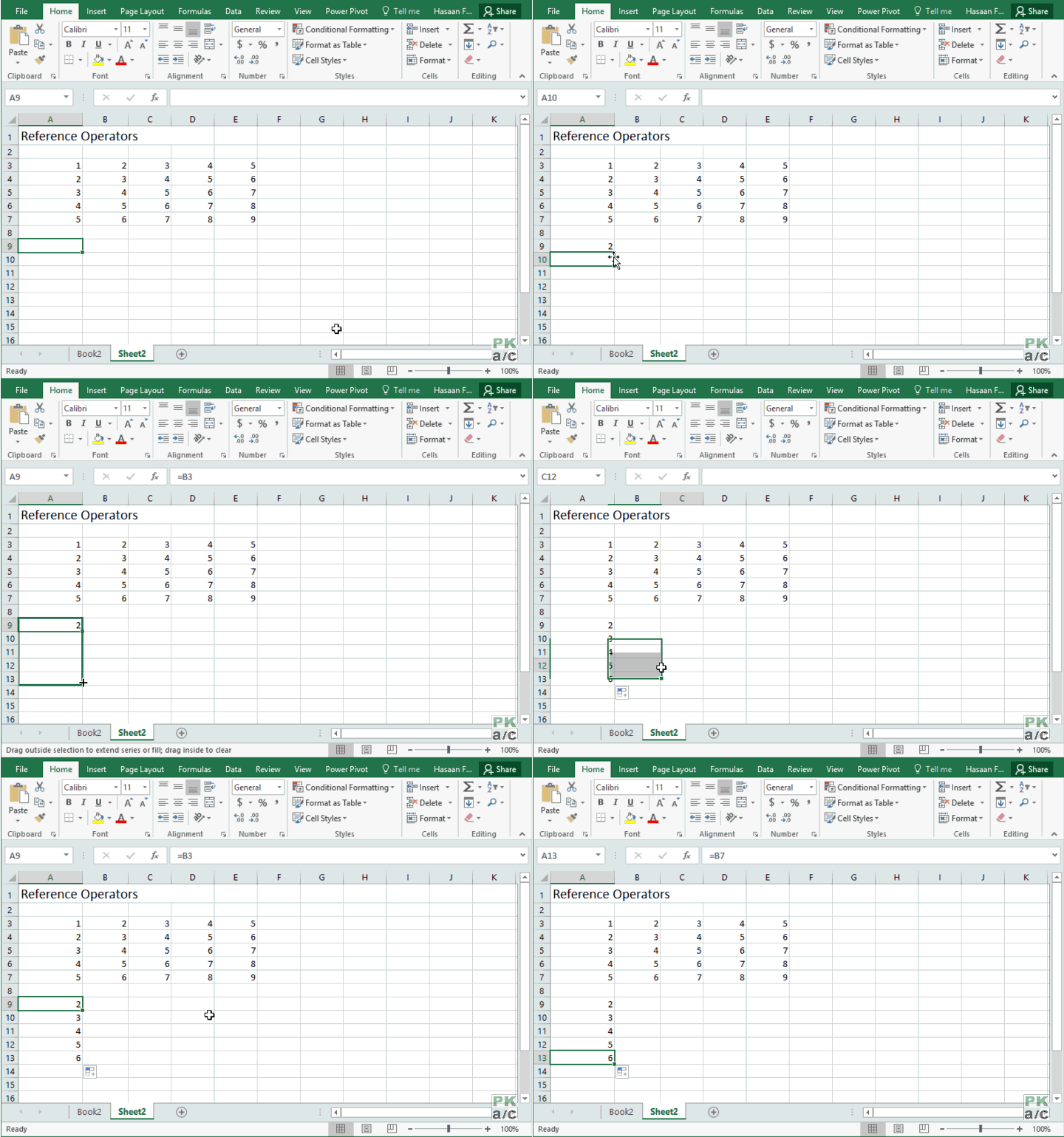
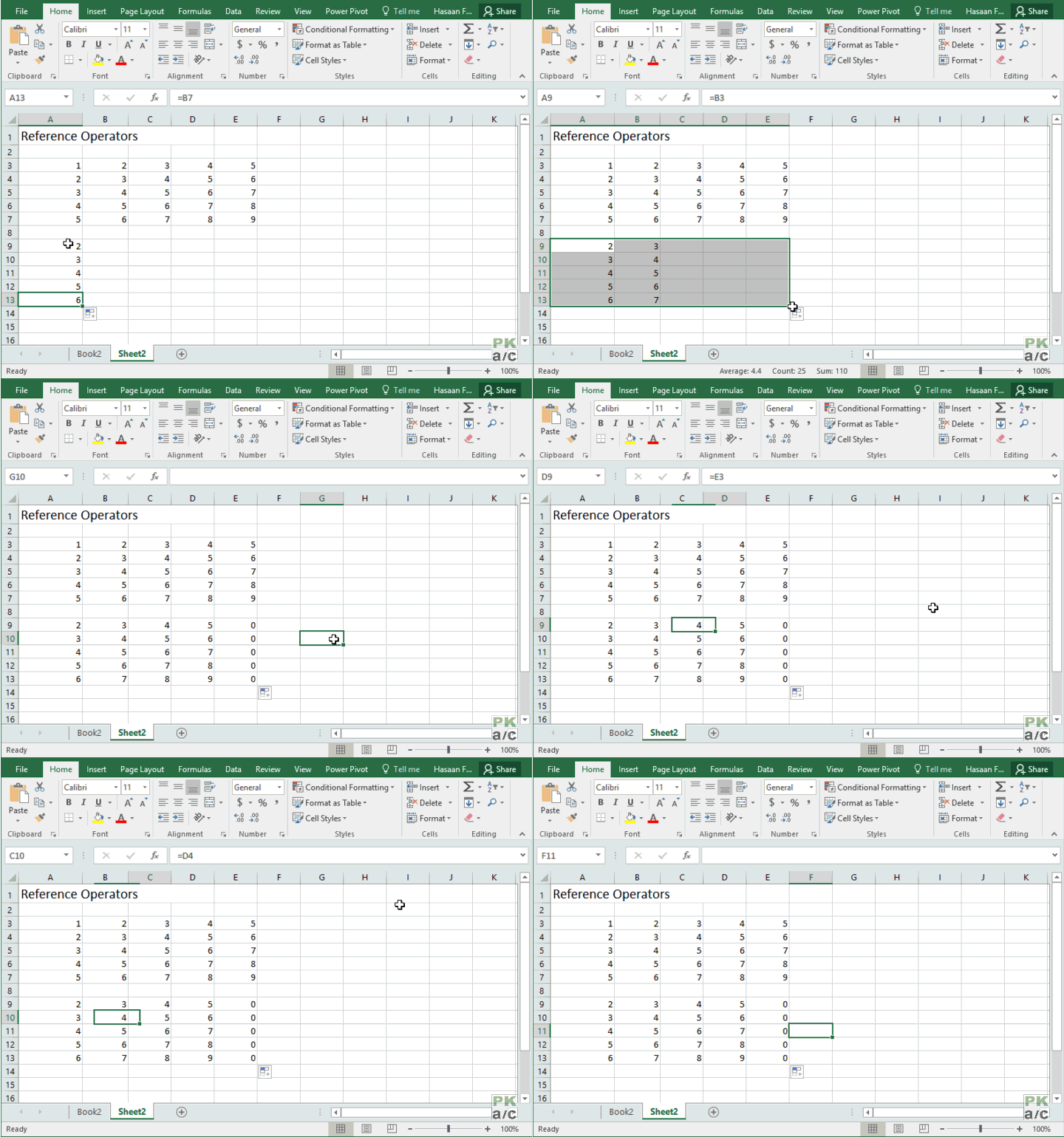
If cell B3 is referred in another cell and fill handle is dragged, Excel will automatically update the address with respect to direction of drag. Observe the following figure closely:

In cell A9 I referred to cell B3 and then dragged the fill handle right. Jumping column C D E and so on. Now later when I highlighted the cells by moving the selector, you can see in the formula bar that reference has changed from B3 to C3, D3, E3 and so on. As F3 and later cells are empty that is why the result is 0.

Now have a look if I drag the fill handle down:

I started again from cell A9 by punching B3 reference again. But this time dragged the fill handle down and trotted down the rows moving over row 10, 11 12 and so on. And if you see in the formula bar while I highlight each cell you will see the address has changed from B3 to B4, B5 and so on.

As I said earlier, if you references are relative Excel will update the address depending on the direction of fill drag.

And if I drag the fill handle to whole region then it will be like this:

Now here you can observe that not only rows has been changed as we go down from cell A9 but also columns have changed as we moved to the right from cell A9.

The reason is BOTH rows and column references were relevant and will change if cell reference is dragged.

So what if we want to:

change only rows and keep columns static: for this we will change the formula as follows; $B3

You can observe that columns remained the same in all the references however, the rows were updated from 3 to 4, 5 and so on.

Change only columns and keep rows static: for this we will change the formula to; B$3

This time row was static but column was changing from B to C D and so on as evidenced by change of value

Make both rows and columns static: for this we will change the formula to; $B$3

By doing so, you can observe that value stayed the same i.e. 2 which is the value of cell B3.

3 Structured reference operators

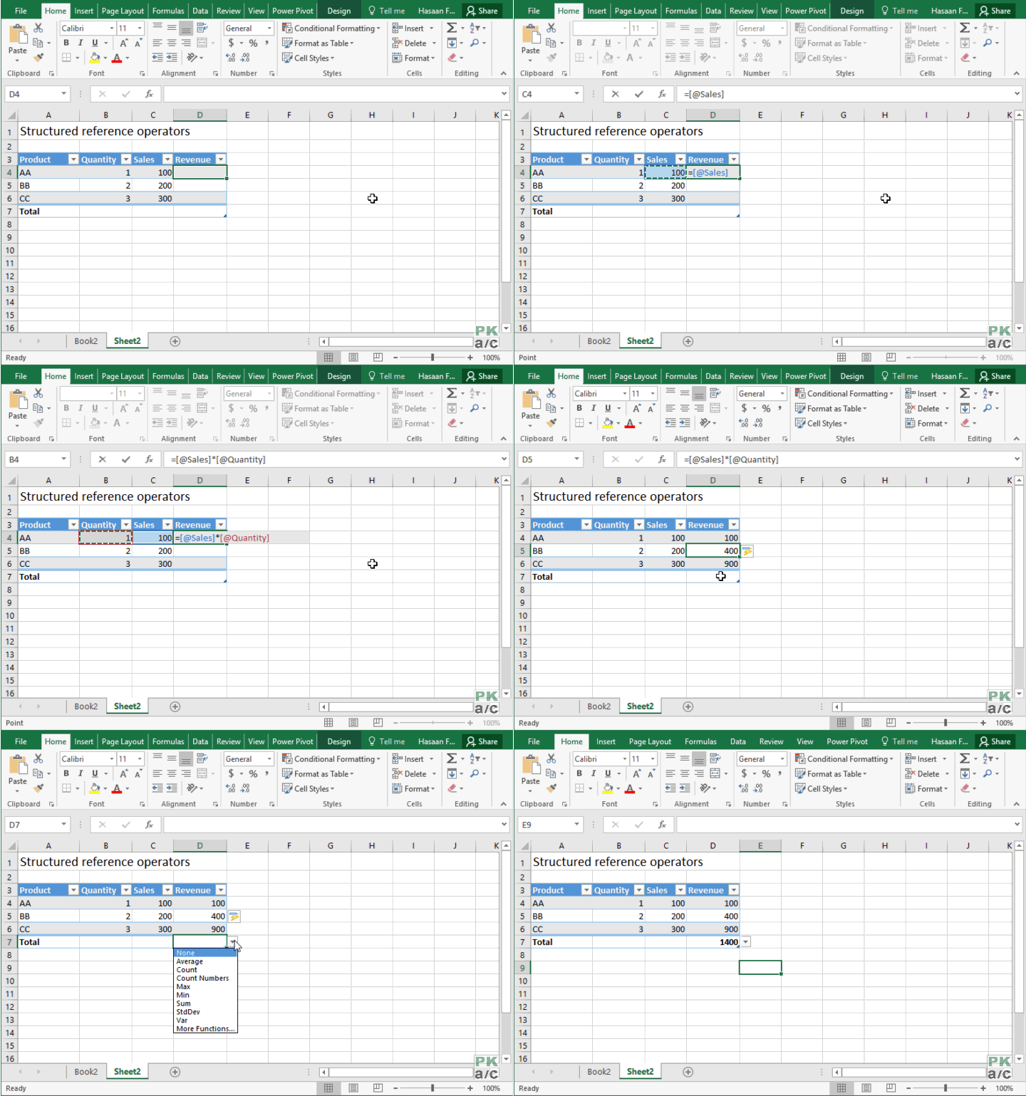
Excel tables are completely different specie when it comes to references. Excel tables can cater normal reference syntax but they have their own system as well called Structured reference system.

Structured reference system gives much more power to the user while writing formulas and enhances readability and understanding. To learn about Excel table and why they are my favourite check out: 20+ Excel Table tricks to turbo charge your data

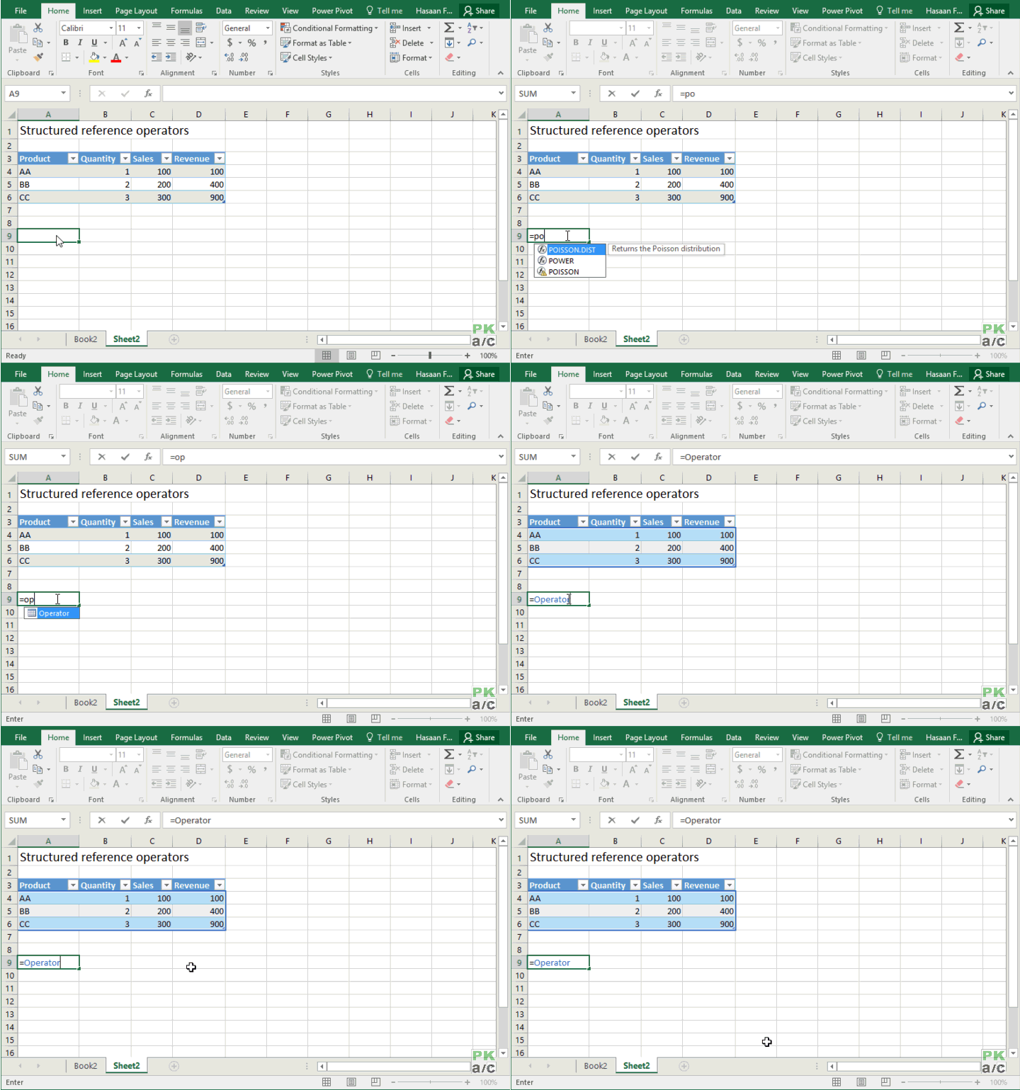
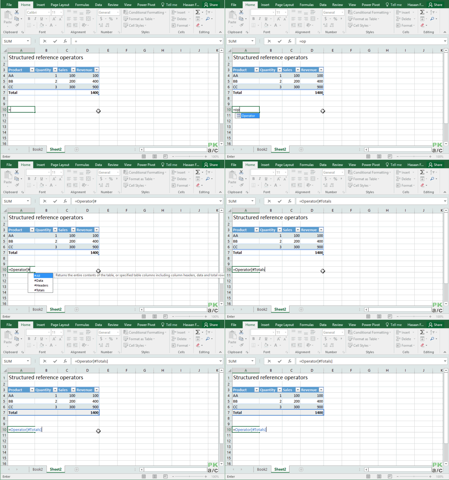
Remember: Every table has its unique name and it can be referred to with its name in the formula instead of mentioning the range. Following is one example in which I have already named the table Operator. After equal sign if I punch “O” you can see the name of table as suggestion. This makes referring to range A3:D6 much easy as I don’t have to use cell reference method.

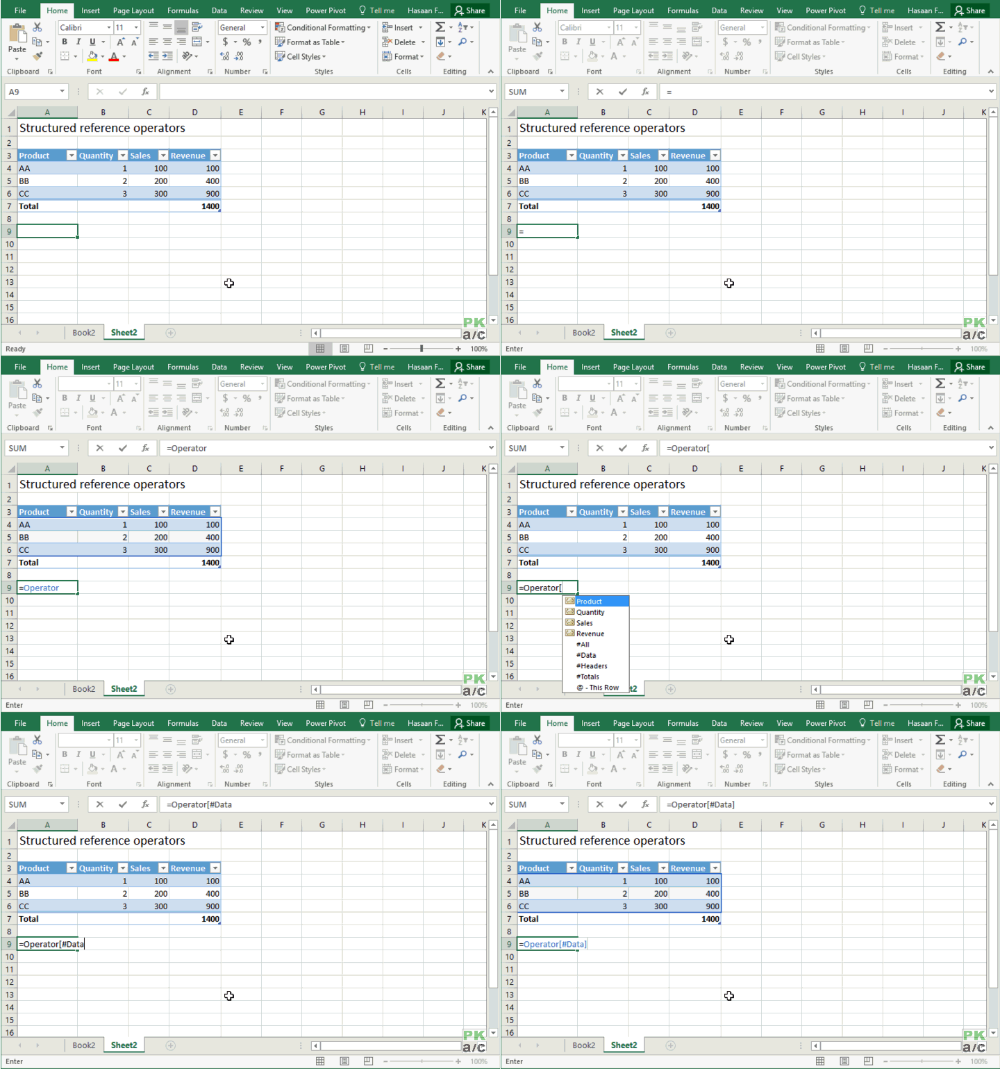
If I mention “Operator” it is enough to refer to table’s data, which you can see enclosed within blue border. Not the whole table though as it excludes header.

3.1 Column Specifier

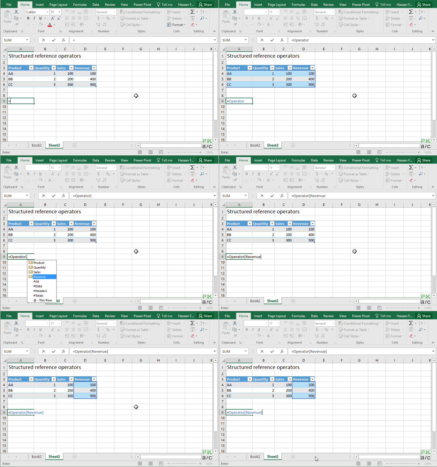
With tables it is very easy to refer to particular column as a whole. Normally we have to give a starting cell and ending cell reference but with tables we have to give just the column header name. To do this we use column specifier which are square brackets.

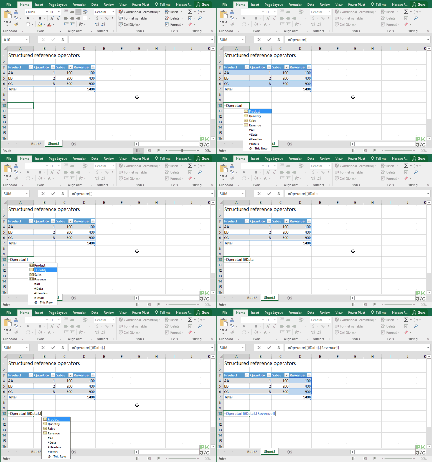
Once you mention the table and insert opening square bracket, Excel will suggest the columns and you can select from the list or type the whole name yourself followed by closing square bracket. In the following figure you can see the data of Revenue column selected by typing: =Operator[Revenue]

3.2 Special Item specifier

Excel tables are like a separate entity that encompass different items in itself. And to refer to each item we use special item specifier. In one table we table we have:

Header row: is at the top of the table which can be turned on/off

Data: is the range where values of different column and rows exist

Total row: an optional row which can be turned on/off and helps in making quick calculations e.g. sum, subtotal etc.

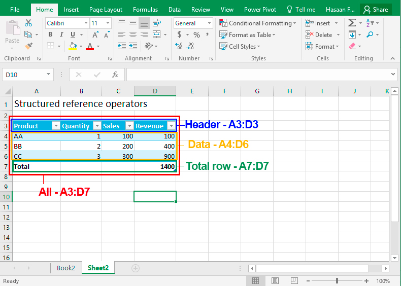
The following figure shows each element labeled for your convenience:

In order to specify each item we have to use special item specifier which are as follows:

#Headers: This is used to specify only header row of the table and its contents. In our case its address is A3:D3 and in formula it is specified as =Operator[#Headers]

#Totals: this specifier is used to mention only the total row of the table. In our example it is A7:D7 and is specified in the formula as: =Operator[#Totals]

#Data: this specifier helps referring to the table’s data which is sandwiched between header row and total row. In our case its address is: A4:D6 and in formula is written as: =Operator[#Data]

#All: So far we saw specifiers that referred to parts of table, what if we want to refer to whole table? In this we use #All specifier. As you can see in the following illustration #All specifier selects the whole table including header and totals row:

3.3 Combiner

Now that you know both column and special item specifier you can mix them together to make even fancier selections. For example if you want to select the data of only revenue column then it will be done using: =Operator[[#Data],[Revenue]]

So in order to combine special item specifier and column specifier you need to separate them with combiner which is coma (,)

3.4 Column range specifier

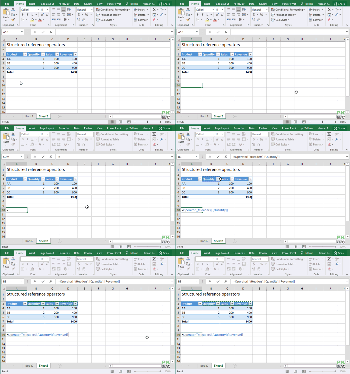
So far we were able to specify either whole rows or data or a row or data of specific column. What if we want to specify multiple columns? In this case we use column range specifier which happens to be the same as usual range operator i.e. colon (:). The only difference is that now we will have column names on the left and right of colon than the usual cell addresses.

Suppose we want to mention the data starting from quantity column until revenue column then it will be done using formula: =Operator[[Quantity]:[Revenue]]

If we want to refer to header row cells only starting from quantity column until revenue then it will be done using: =Operator[[#Headers],[Quantity]:[Revenue]]

3.5 Current row specifier

Until now we have made quite a progress in understanding not only operators used in structured references but also understand how structured reference system is different from usual system in use.

Lets say I want to calculate the revenue of sales by multiplying the values of quantity column and sales column. To get this done I want to multiple the value in each row of quantity with the respective row value in sales column. To do this we will use this formula in revenue column: =[@Sales]*[@Quantity]

The @ symbol makes sure that each row item is considered instead of whole column.

3.6 Escape character

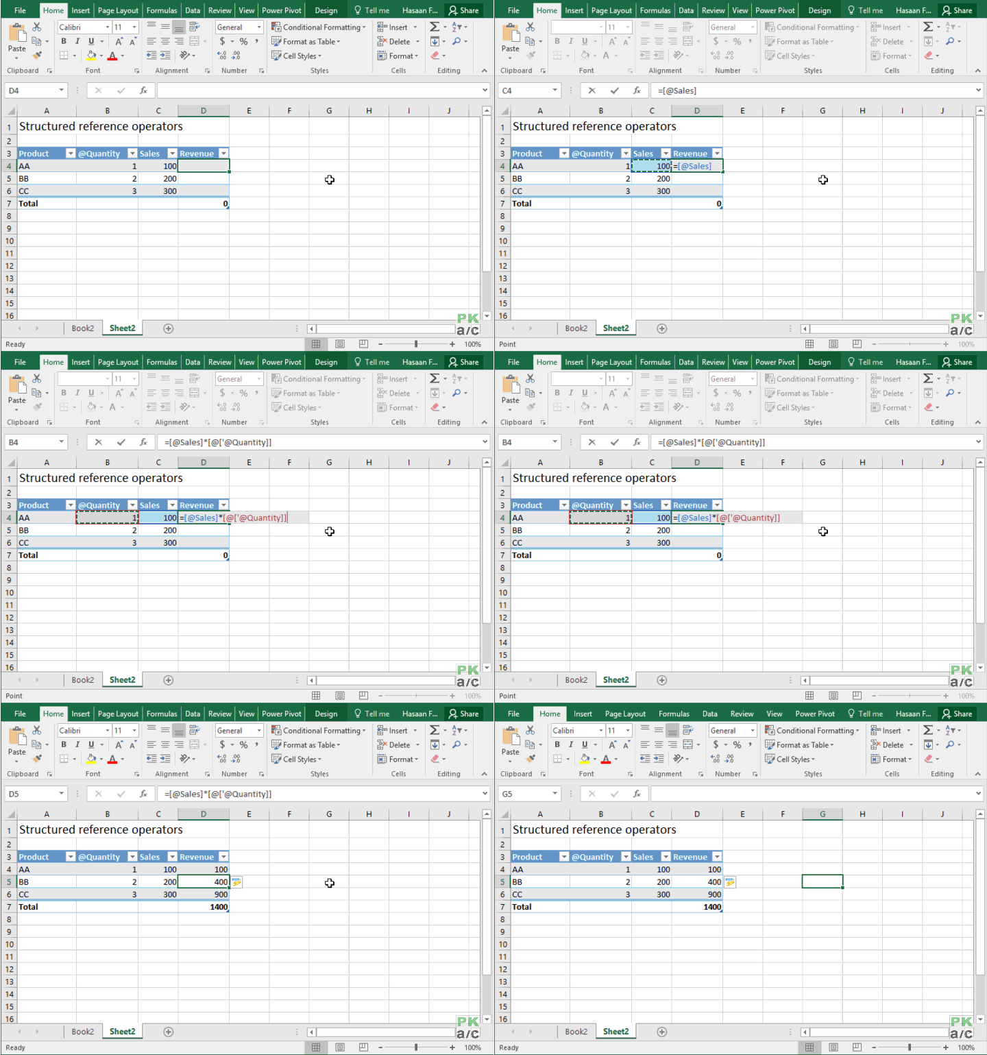
In the above examples we learnt that @ # or , characters have special use and Excel considers them as operator. What if our headers have any of such characters? In such situations naming the column can be difficult.

For example if one column is named as @Quantity. If we refer to such column with @ then Excel will treat it as row specifier whereas we want to use it as part of name. To get around it you simply have you put apostrophe before such characters and Excel will not consider them as specifier.

Have a look at the following illustration:

As one column is named as @Quantity then our revenue calculation formula will be like this: =[@Sales]*[@[‘@Quantity]]

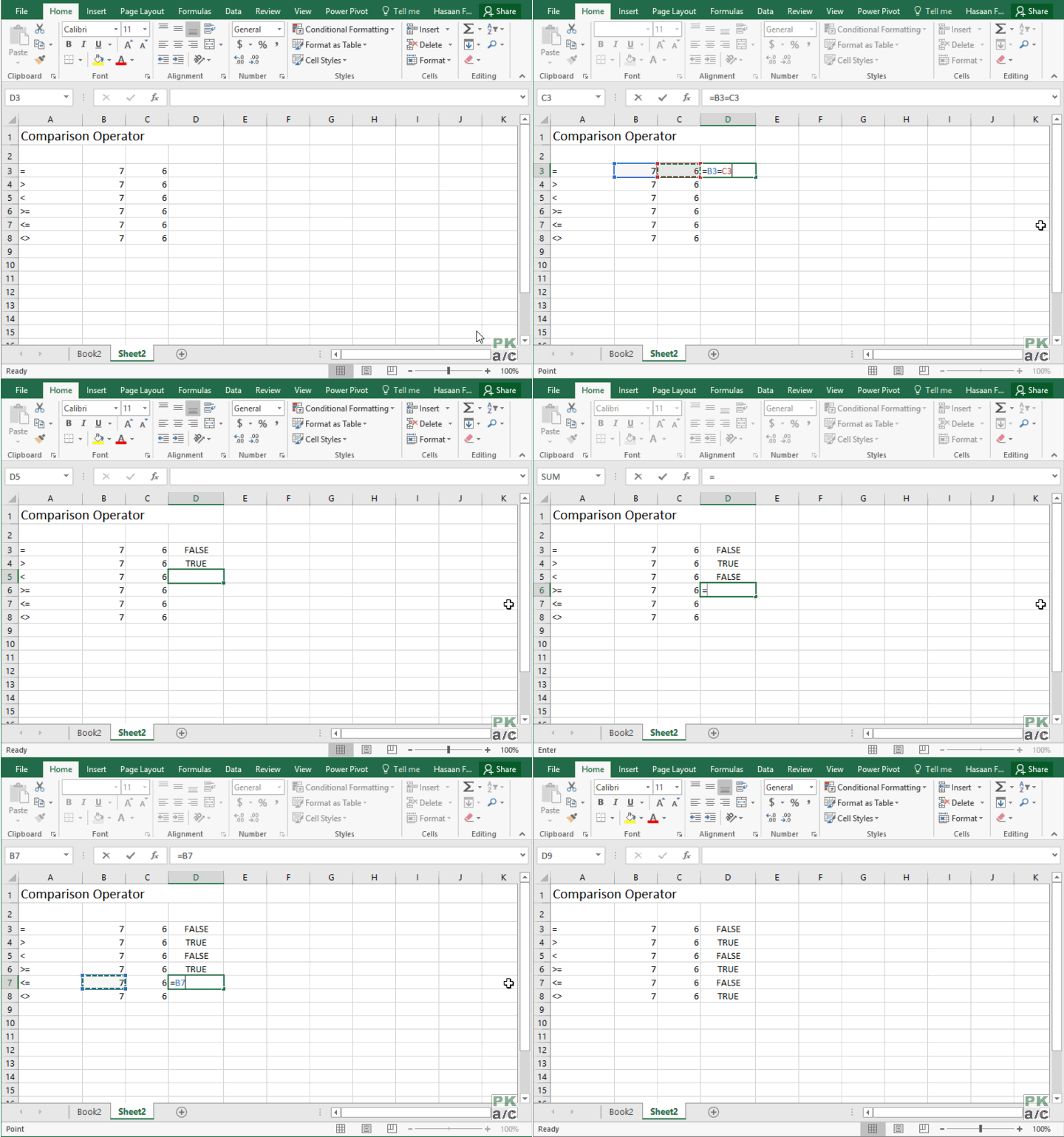
4 Comparison Operators

Like basic arithmetic operators, comparison operators work the same way as we use them in our daily lives. They help us compare the data and give us result either in TRUE or FALSE.

5 Concatenation operator

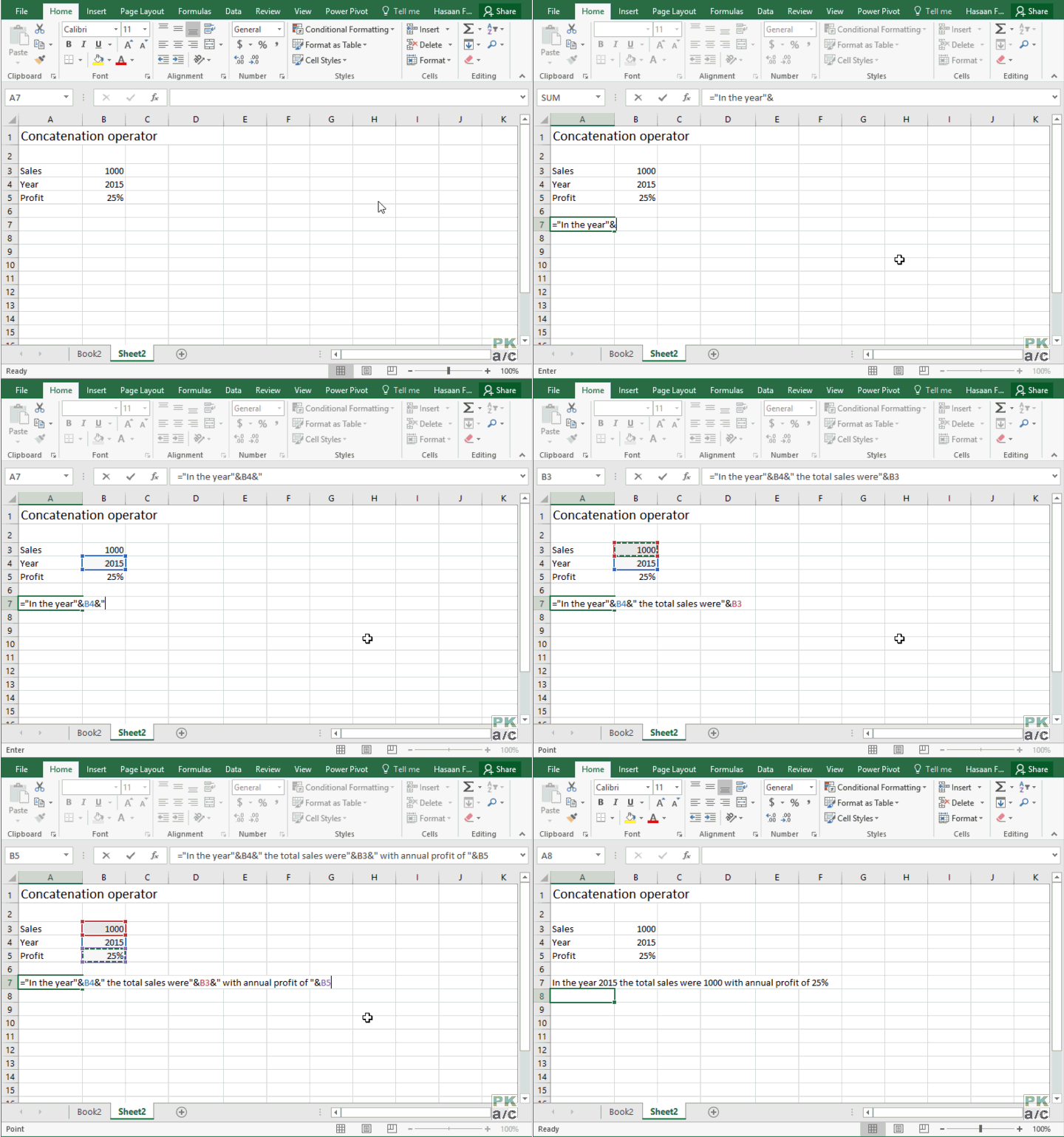
Often we have our data scattered in different cells. In order to combine the data to show as one textual string, we can use CONCATENATE function or its short form (&) to join the data from different cells.

In the following illustration we have data in three cells and we also want to add few words from our own. We will do this using concatenation operator

6 Wildcard operators

These operators help in searching something and can be used either in Find & Replace feature, Filters or select formulas of Excel.

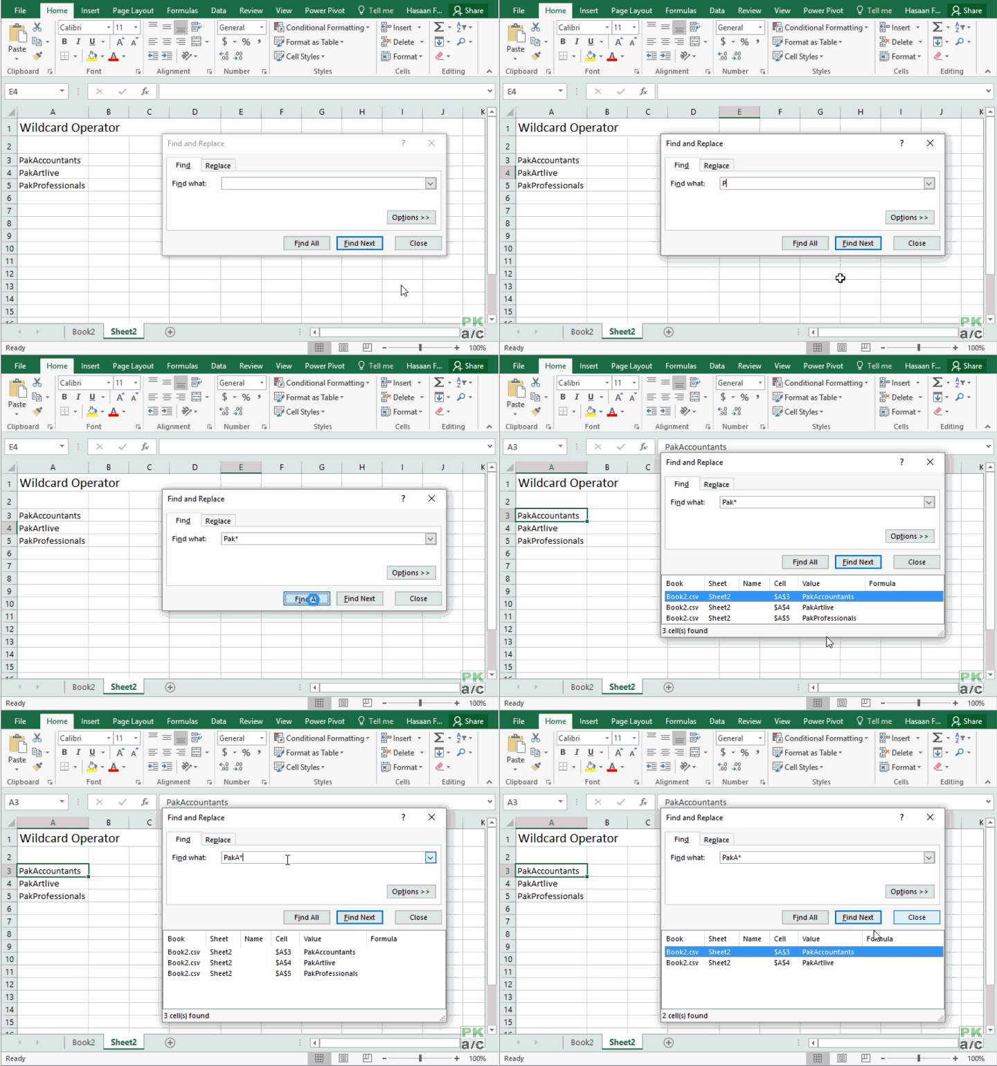
Asterisk: if used returns a matching results before, after or within string. For example you have PakAccountants, PakArtlive, PakProfessionals etc

If you put Pak* in the search box and run find it will select all three because all three start with Pak and asterisk will get all such results that start with Pak. But if you make it PakA* then it will select only first two as the last one does not match after “PakA” string.

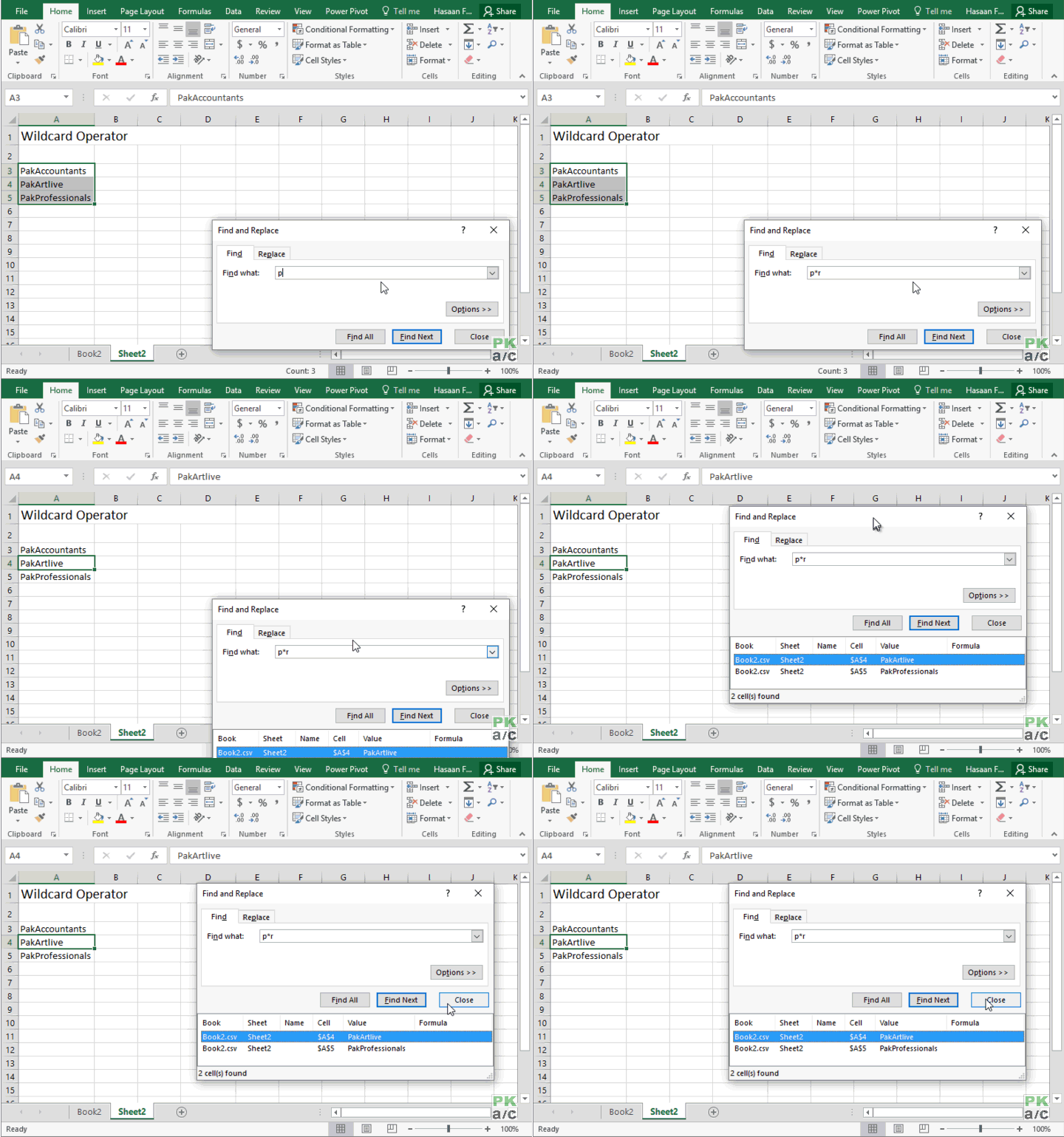
If asterisk is enclosed within two strings then it will fetch all such results that contain both strings. For example if we search p*r then it will fetch both PakArtlive and PakProfessionals:

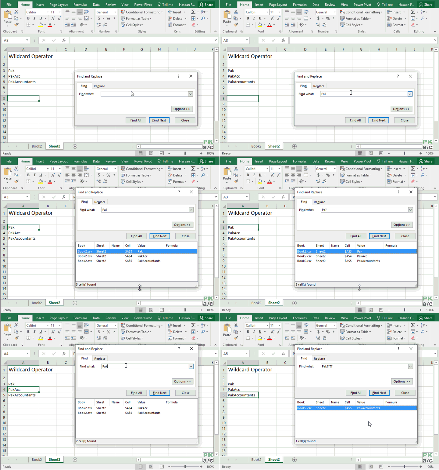
Question: If used is considered as a single character. Suppose you have; Pak, PakAcc, PakAccountants.

In the search box if you mention Pa? then it will select all the records that have ATLEAST one character after “Pa”. Similarly if you put Pak? then find will result only in selecting PakAcc and PakAccountants.

If you enclose it within two strings then again it will work as single character. If you put P?k then it will find all the records that have P and also have one character between P and K as following example shows in which Paak wasn’t selected:

Tilde: This is an escape character that forces * and ? to be considered as normal characters instead of wildcards in searches and formulas. I have written a detailed tutorial on this and please consider reading it: “Call Tilde” to tame Excel Wildcards – Find and Replace Wildcard Characters [Quick Tip]

Right so you had a great dost of excel operators!. So now that we know what they are and how to use them, how are you using or planning to use them? Let me know in the comments below and we will definitely be learning more!