Stock Ageing Analysis Reports using Excel – How To

 Stock Ageing Analysis Reports using Excel – How To

Stock is one of the most important investment made by the entity. Optimum quantity and turnover period is essential for entity to be successful. Faster the conversion, better the prospects for entity as inventories not converting to sales mean stuck-up cash.

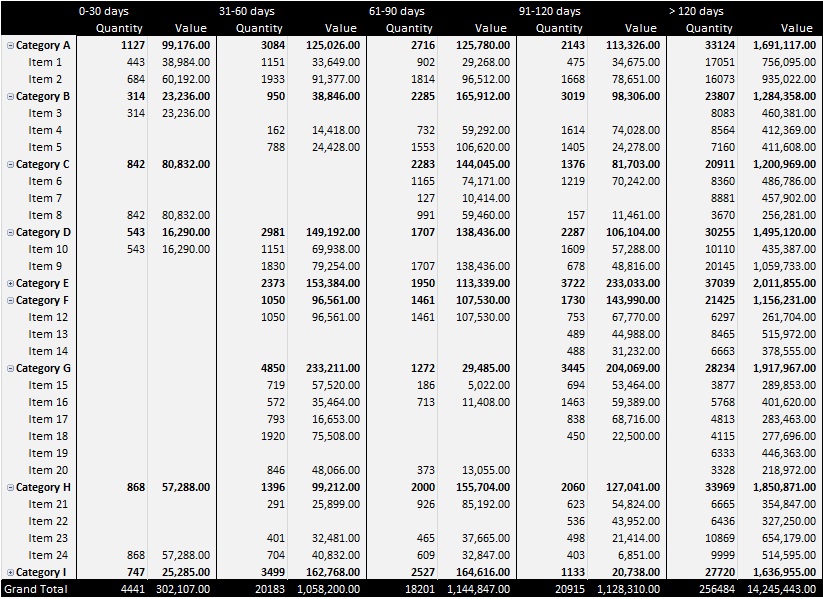
To monitor stock and identify slow moving inventory or that is not converting, stock ageing analysis reports are made. The most common stock ageing analysis involve determining the age of product on the basis of data of purchase and particular date i.e. today’s date or any other date. Following is the stock ageing analysis based on today’s date:

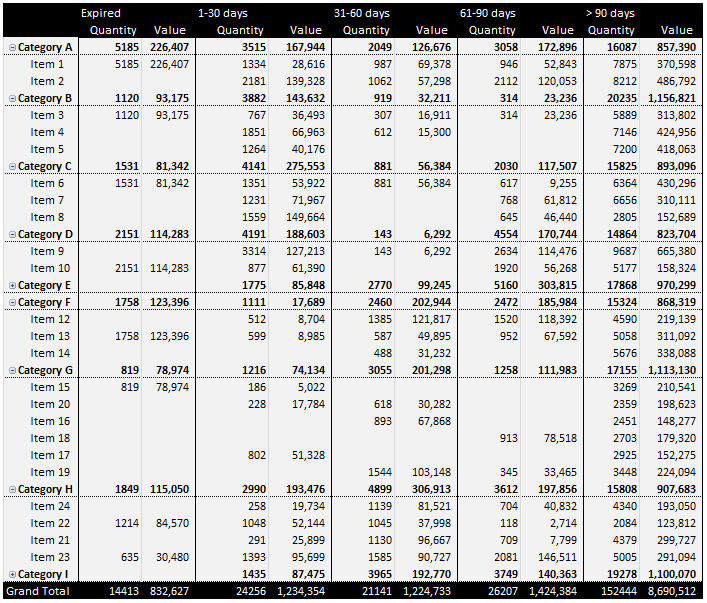
However, we can prepare ageing reports based on expiry date of stock to identify any expired stock and how many units (with their value) have what time remaining until expiry. Following is the stock ageing analysis based on inventory’s expiry date:

Lets understand how it is done.

View Contents [hide]

Stock aging analysis using Excel – Step by step

Step 1: Download this tutorial workbook that contains the data that we will use for stock aging reports. It has worksheet with several columns and data range already converted to Excel table.

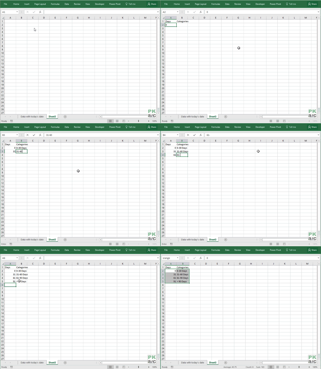
Step 2: Insert a new worksheet and mention the categories in which you want to produce aging analysis report and the corresponding length of time as shown below and skipping the heading select the range and give it a name using name box. I used ‘srange’

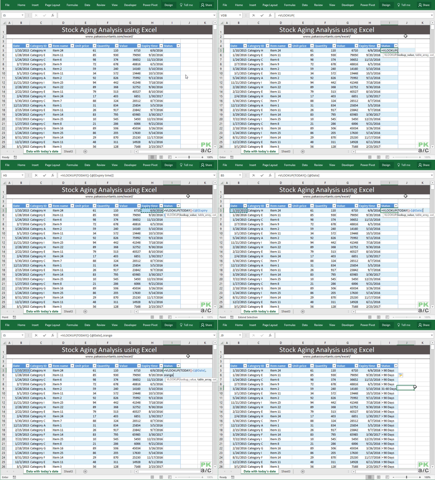
Step 3: Go to cell I4 and enter the heading “Status”. Click enter and it will automatically insert a new column to existing table.

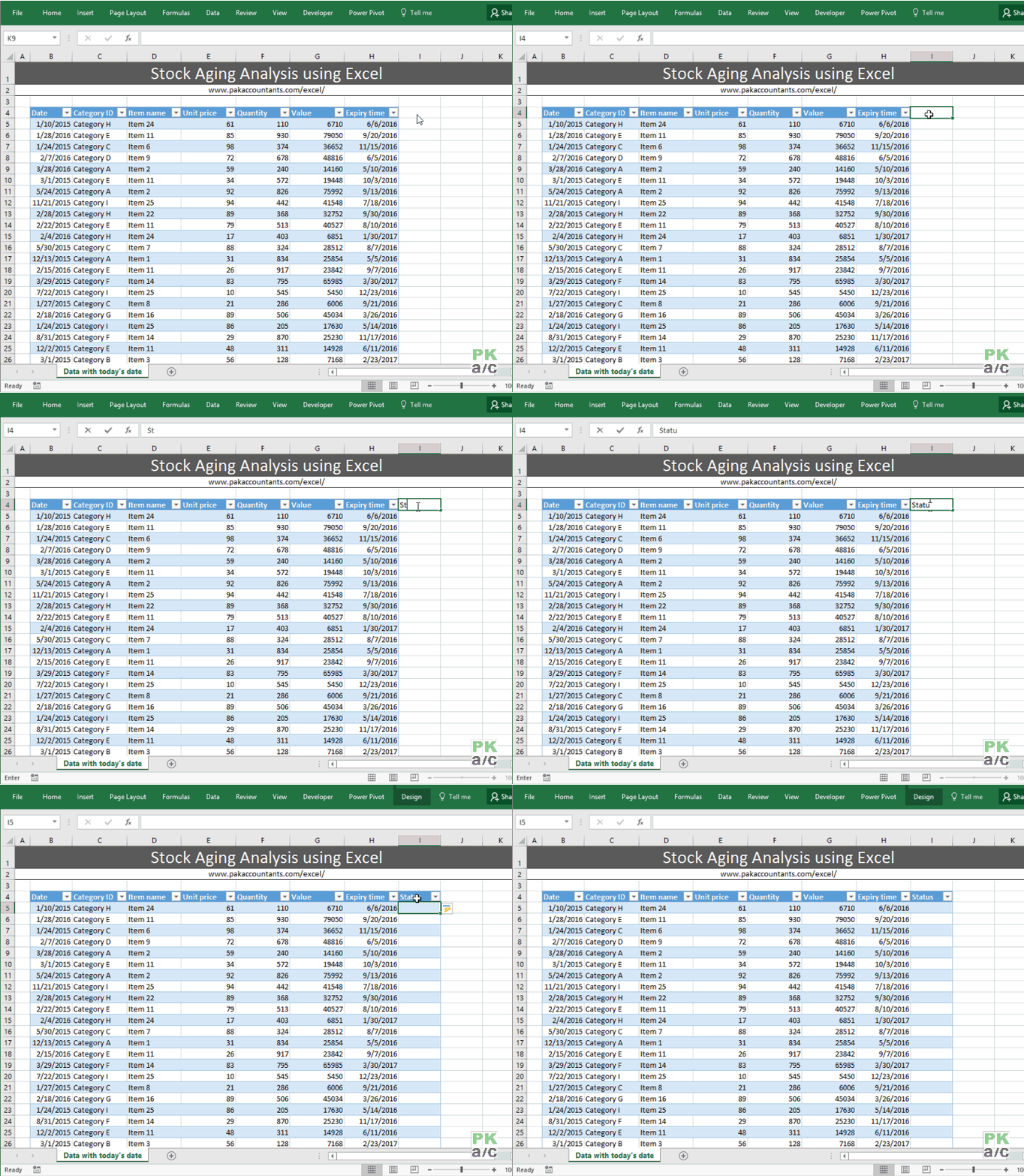
Step 4: Put this formula in cell I5 and press Enter key it will automatically populate:

=VLOOKUP(TODAY()-[@Date],srange,2,TRUE)

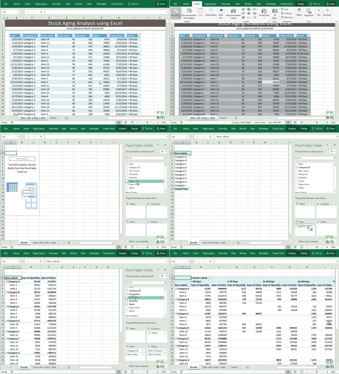
Step 5: Select the table by having an active cell within table and hitting CTRL+A combo. Then go to Insert tab > tables group > click pivot table button. A dialogue box will appear click OK. It will insert the pivot table in the new worksheet.

Step 6: Move the fields to quadrants in the following sequence:

1. To rows quadrant:
   1. Category ID
   2. Item name
2. To values quadrant:
   1. Quantity
   2. Value
3. To column quadrant:
   1. Status (above already inserted values field)

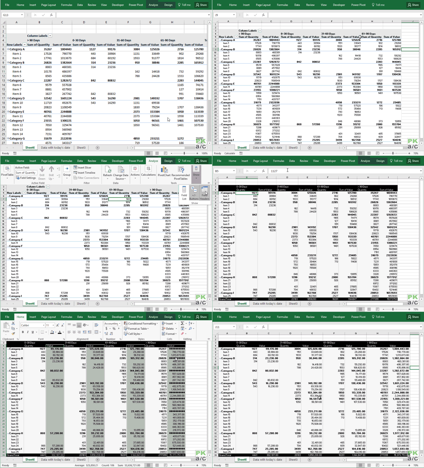
Step 7: Now we need to do few cosmetic changes and its all done:

• Fixing the “Sum of…” part. Simply remove the part from the formula bar and at the end insert space bar so that Excel don’t thrown an error.
• Move the column by holding on to the edge of “status” field in the pivot table to appropriate location. In my case “> 90 Days” column was appearing as first which should be last. So I moved it to the end.
• Change the style to your liking.
• Turn off header and grand totals if you like.

Here is the how it looks in the end with little more styling using borders:

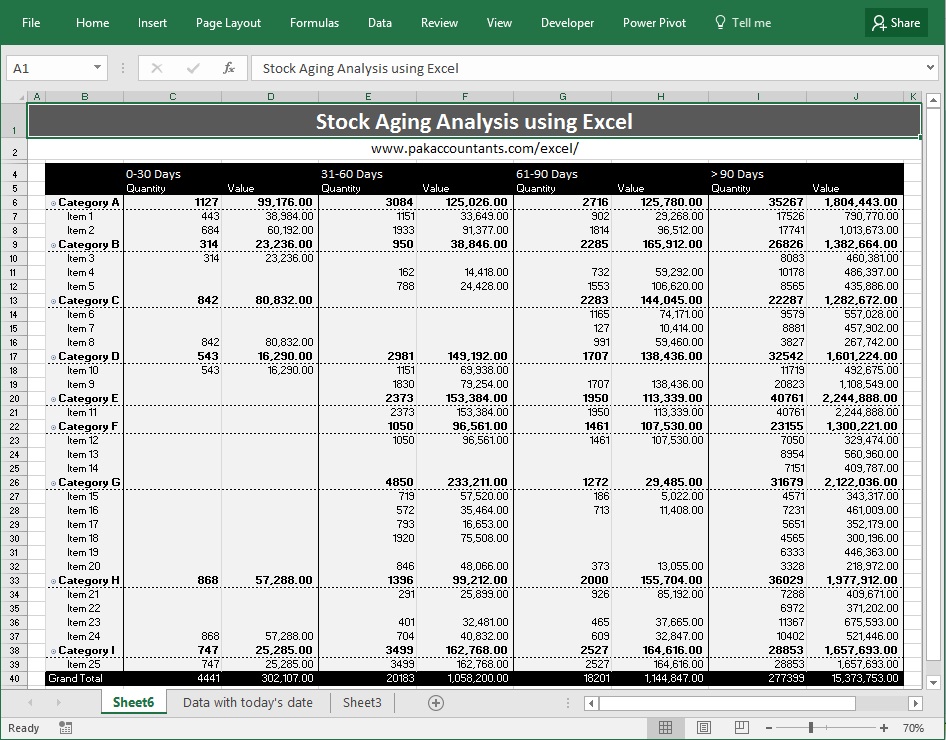
Don’t worry about the font size, just to make it fit here, I have intentionally kept it at 70% so that you can see the whole report. Had it on 100% and everything is normal.

Bonus tip: Dynamic aging slabs

In the above solution we used four slabs of aging i.e:

1. 0-30
2. 31-60
3. 61-90
4. > 91

What if we want to increase or decrease the slabs? We can definitely change the slabs and change the formula accordingly, however we can make it dynamic to great extent. For this we need to make few changes one time only.

Go to the worksheet where slabs were mentioned and change that data range to table. I named this table “slabs”

Now go to status column and replace the old formula with the following:

=VLOOKUP(TODAY()-[@Date],slabs,2,TRUE)

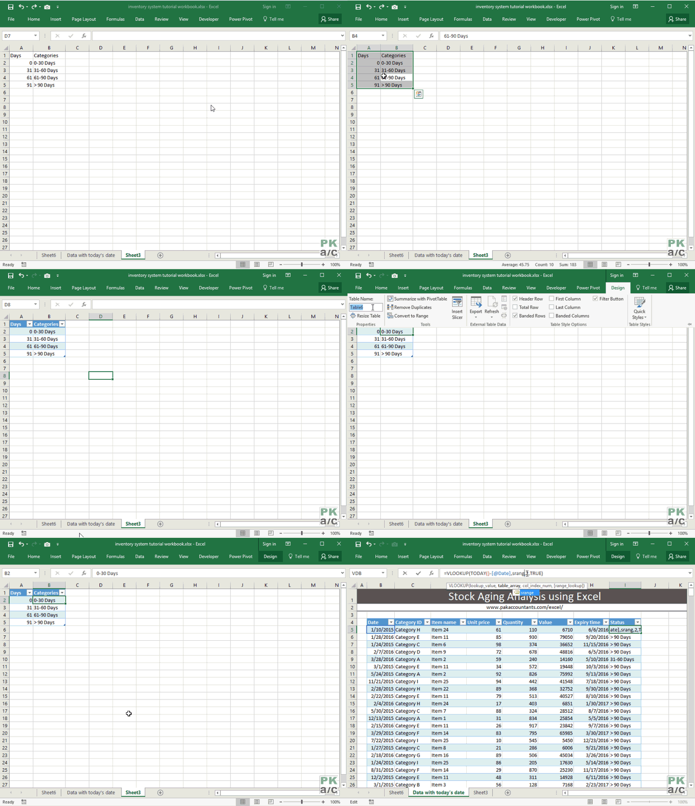
Now if you change the slabs, your aging report will update at the push of a button! Remember, currently we have 4 slabs.

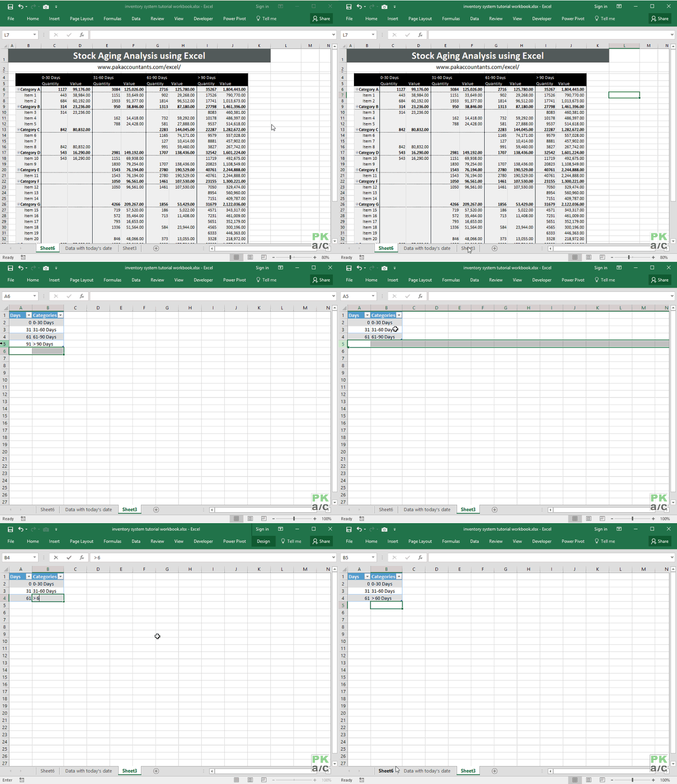
Here is if I remove one slab and refresh the pivot table:

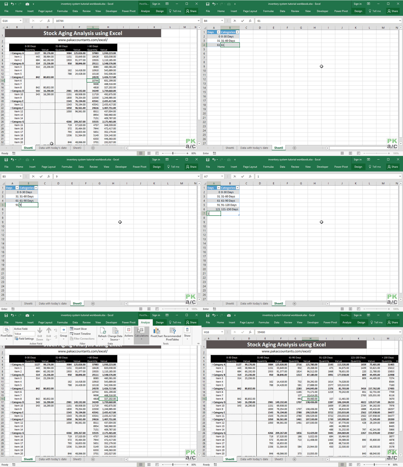
And here is if I add more slabs and then refresh the stock aging report:

So here you have your own stock aging analysis report WITH dynamic slabs! HiFIVE!