Rounding to nearest 1, 10 or 100 in Excel – How To

Don’t be frightened I am not giving you any fifth graders’ challenge. But in real life you might be facing similar situation where you have a stack of numbers that require to be rounded either to nearest dollar or nearest 10 or 100.

So how would you do it in Excel? Well you don’t really have to bite your nails out to get this job done. Excel gives you not ONE not TWO but THREE functions to get around rounding named ROUND, ROUNDUP and ROUNDDOWN.

Syntax of all three is similar and as the names suggest ROUND function rounds as normal, ROUNDUP function rounds the number up whereas ROUNDDOWN rounds the number down.

ROUND = (number,num_digits)
ROUNDUP = (number,num_digits)
ROUNDDOWN = (number,num_digits)

Whereas;

number: the number you want to round which can be a number or a cell reference containing a number.

num_digits: the number of digits or places you want Excel to round the number which can be a positive number, a zero or a negative number.

Yes you read it right. Many don’t know that you can use negative numbers as num_digits argument.

In short,

• Positive numbers will affect the digits at the right of the decimal. For example if you put “2” then it means you want the number to be rounded to 2 decimal places
• Zero will ask the Excel to shed of all the decimal numbers and round the number to nearest whole number
• Negative numbers on the other hand will affect the numbers at the left of the decimal. For example if you use -1 then it means you want the number to be rounded to nearest 10.

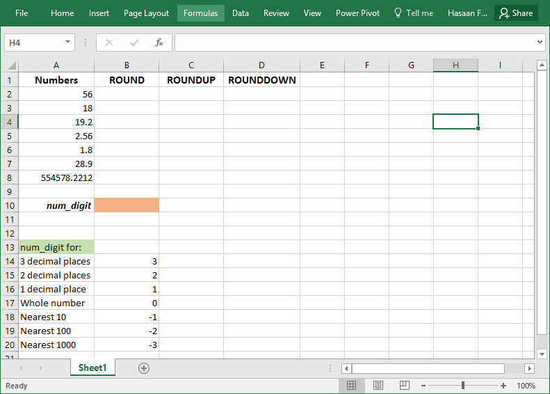
Say you have following numbers: 56, 18, 19.2, 2.56, 1.8, 28.9, 554578.2212

And your rounding requirement can be either of these:

1. Round, round up/down to 2 decimal places
2. Round, round up/down to 1 decimal place
3. Round, round up/down to nearest whole number
4. Round, round up/down to nearest 10
5. Round, round up/down to nearest 100

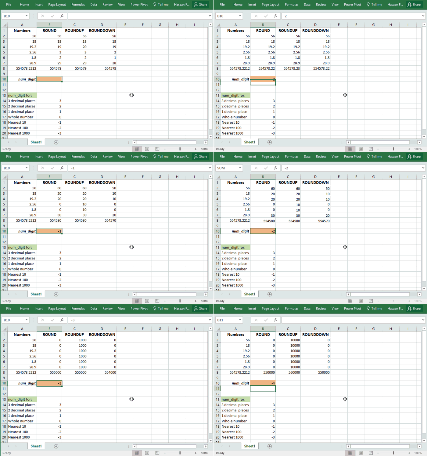
To quickly understand and compare the output of all three functions I have arranged the data as follows:

I put the formulas as follows:

Cell B2: =ROUND(A2,$B$10)
Cell C2: =ROUNDUP(A2,$B$10)
Cell D2: =ROUNDDOWN(A2,$B$10)

Important: I used cell B10 as a num_digit argument so that I can change it to show it affects the rounding function.

Now in cell B10 you can type in the number to make the rounding as you desire. Remember the number you use will affect the rounding process and nature:

Important: If nothing is mentioned in the cell B10 then Excel will conduct the calculation by assuming “0” as the argument. But while writing the formula directly you have to provide something to make the formula work.

So here you have an extra dose on Excel and Rounding together. Just remember that you can use negative numbers in ROUND functions and it gets you nearest of 10 or 100 or 1000 or whatever you fancy.

Liked it? Pin it!