Pivot data using Power Query to show text values – Data Restructuring using Excel – How To

The ones who make reports on daily basis using Excel can understand how important the data is and how equally important data structure is. With data structure I meant the way data is arranged and made available for processing.

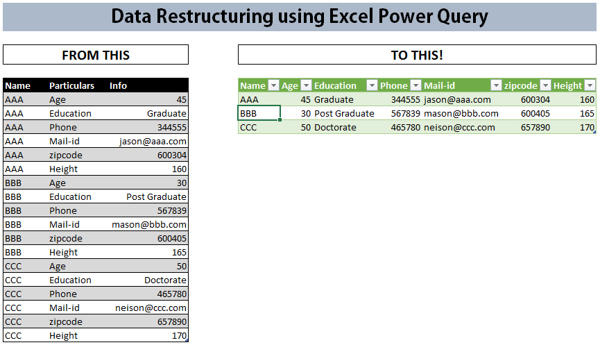
Today we will discuss a little about data restructuring and different features/tools Excel offers with few examples and tutorials. Later we will learn a cool technique to restructure our data using power query as pivot table failed to deliver us. Here is snapshot of what we will learn today:

 

So lets start with few words on data restructuring.

We have several tools and features available in Excel to process data in many different ways possible. Sometimes we use basic features like transpose to reshape our data.

Read: 5 Ways to Transpose in Excel – Shifting Columns to Rows or Rows to Columns

Pivot table is one of the best tool that actually arranges the data for us but it also require data to be structured in specific manner before it can be fed to pivot table.

Read: Excel Pivot Table – Introduction for Absolute Beginners – [Part 1] + [Part 2]

But even for pivot table, we need to have data structured in the right manner before it is fed to make pivot reports or simply pivot table.

Read: Prepare (Normalize) the data for Pivot Tables using Power Query

And sometimes we need to combine the data from two different sources to make one data range so that it is processed as one report

Read: Combine or Append data in one table from multiple sources using Power Query in Excel

And this isn’t the end. There is a lot more Excel can offer. I have given only few examples of fraction of things possible with Excel. I haven’t even mentioned Powerpivot yet.

Now lets move on to today’s tutorial in which we will learn how to restructure our data using power query because pivot table isn’t helping.

Here is the data once again:

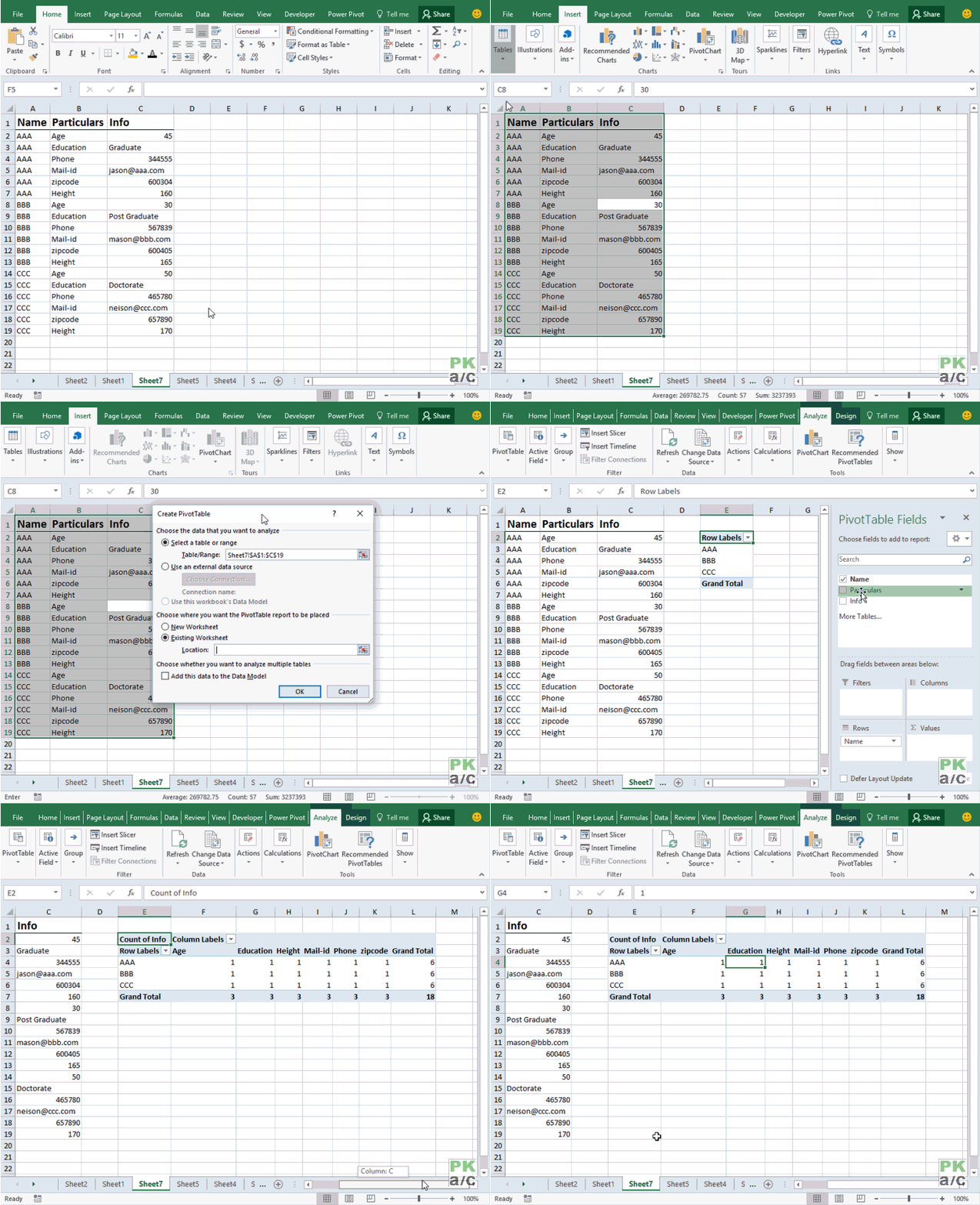
Now what we want is that for each name other particulars are along the column so that it sites nicely flat and easy to read as well. All this could have been achieved with pivot table if it somehow allows us to display text values from the data. But pivot tables are made to process numbers and they don’t take text as pivot table summarizes in counts, sums, averages etc as the following illustration shows:

So the solution is to use power query. In older versions of Excel it comes as a plugin which you can download but in later versions it is part of Excel. So here is the step by step to get the required shape of data.

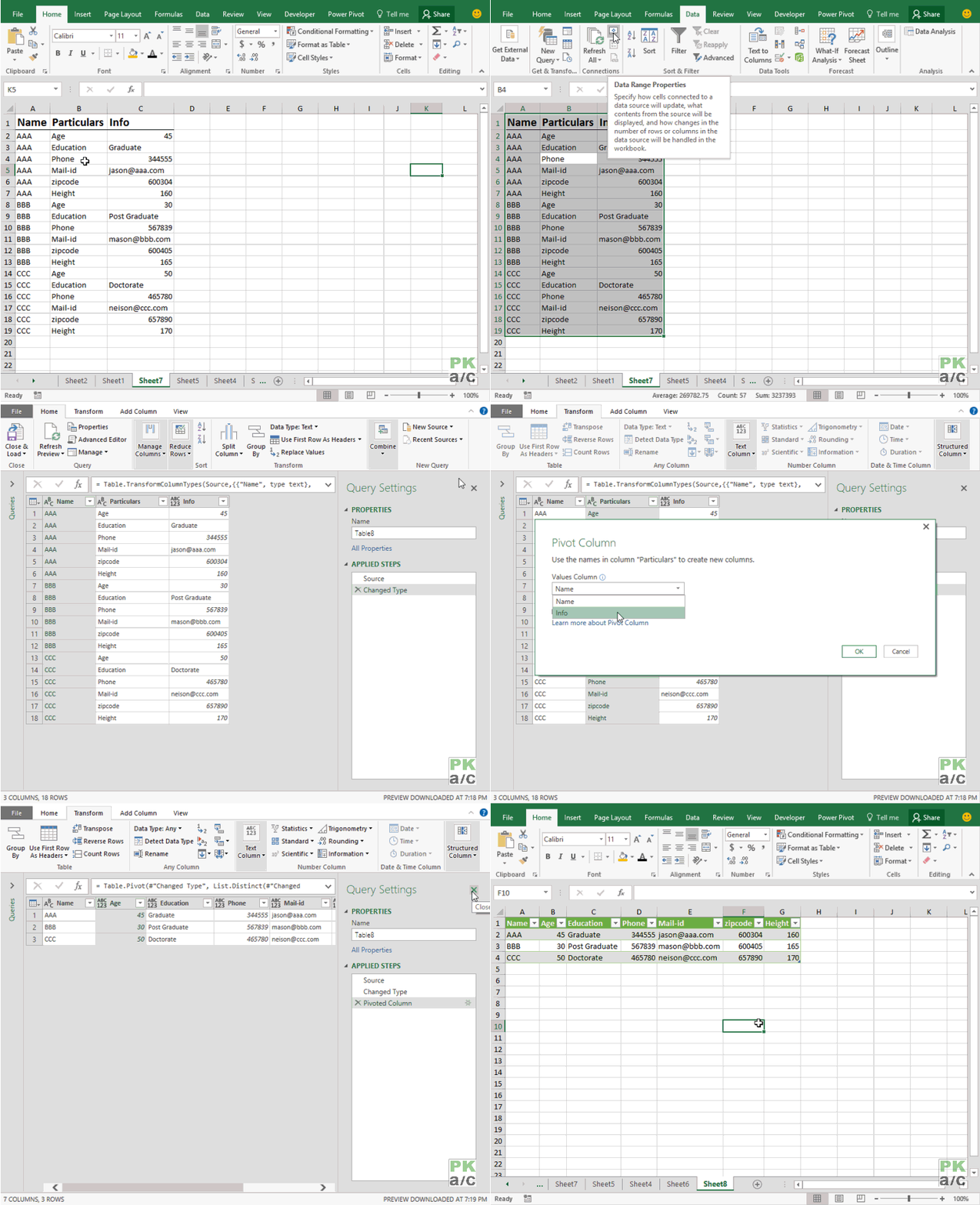
Step 1: Select the data range > go to Data tab > get and transform group > click from table. A dialogue box will appear that will change your data range to table if its not already a table. Click OK.

Step 2: Query editor will initiate and load your data in power query for processing.

Now what we want is to pivot particular column so that it each particular shows in individual column as headers with info items as content.

Have the particular column selected or activated by clicking once, it will turn green if its activated/selected.

Click transform tab > in “any column” group > click pivot column.

Step 3: From the dialogue box that appears under “Value column” select Info from the list. We are basically mentioning which column to use to take values for each particular headers. 

Step 4: Click advanced options accordian to expand it and select don’t aggregate from the list. This will instantly restructure your data as we desire.

Step 5: Click Home tab > click close and load button and it will insert the data in new worksheet.

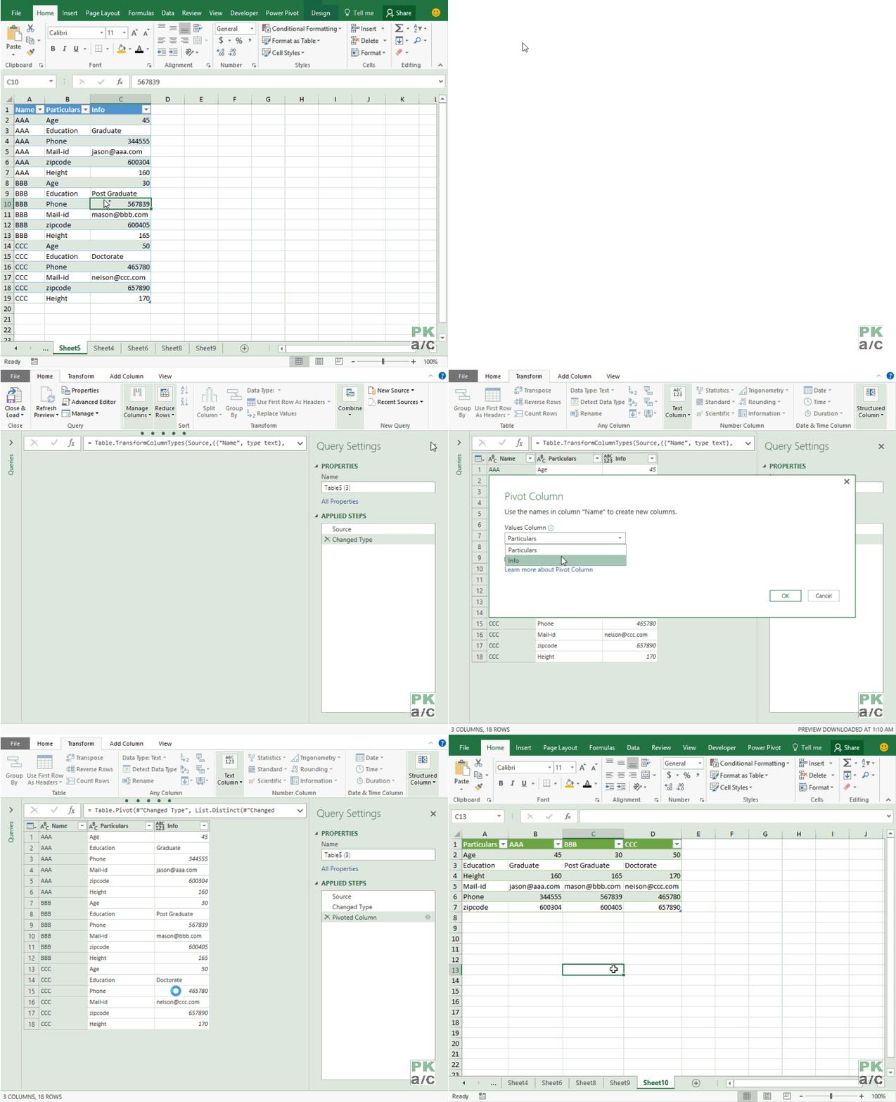
Now that we have learnt how to use power query then we can pivot the data in different ways. Like if you want names to be the headers and particulars along the rows under each name then you simply have to select name column and pivot it with “Info” as value column.

So there you have it! A new trick to try for you. Let me know what method you use normally to restructure data if you have to in the comment section.