Make Budgets in Excel with Expenditure Limit – Budget Ceiling using Data Validation [How To]

Budgets help control the expenditures even before they actually incur. The concept of budget is to provide a ceiling or cap to expenditures so that departments or cost centers don’t exceed a certain limit.

If we have to draw a budget in Excel then we can use data validation to limit the total spending. And intimate the user that expenditure cannot exceed authorized limit.

Lets say we have a total budget of 7.6 million and allocated as follows:

Admin: 20%
Selling: 10%
Finance: 5%
Research: 25%
Training: 15%
Capital: 25%

Now it depends on the policy of the entity if particular expenditure head can exceed the allocated amount or not. Sometimes particular head can go over limit but the total budget is strictly kept to authorized amount. In this case we need such Excel solution in which if:

• particular expenditure head goes over limit then a soft intimation is given
• but keeping the total expenditure strictly up to the total mentioned.

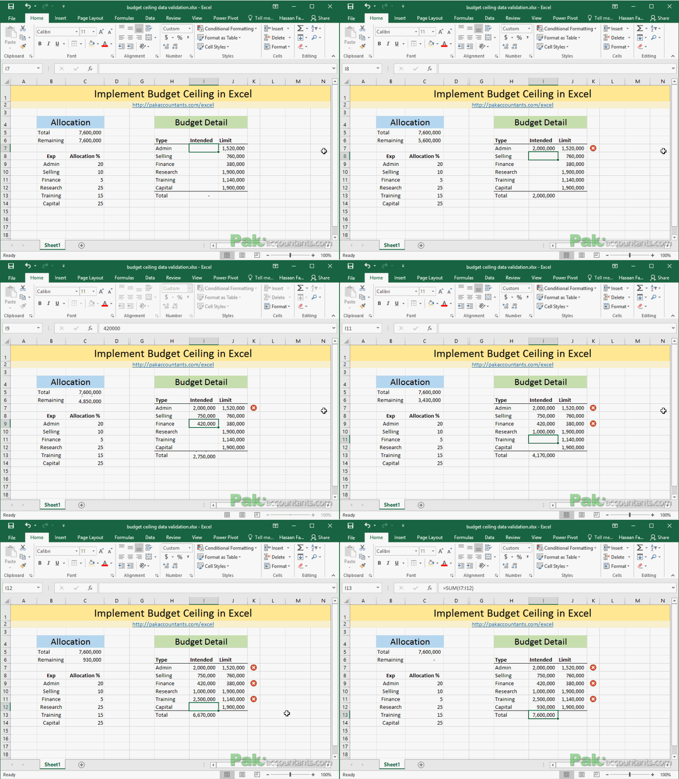
To achieve this, I used conditional formatting for the first requirement but data validation for the second. And final result is as follows:

In the illustration above you can see that if particular head exceeds its allowed limit then a sign appears to the right but it does not hinder the calculation however, if expenditure exceeds the remaining budget then Excel restricts the input. The following step by step explains how to do it.

Budgets with Limits – Step by Step

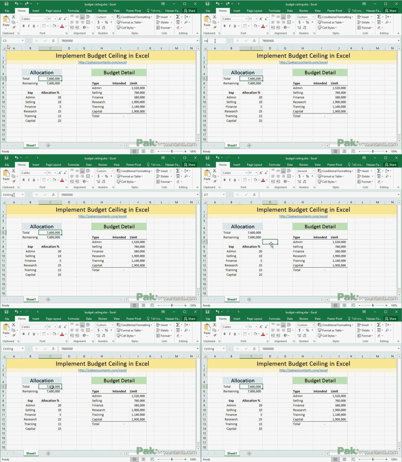
Step 1: Download this tutorial workbook that provides you with basic data and open it in your Excel program.

Step 2: Select the cell C5 and in the address box type Ceiling and press Enter key. This cell now has a name.

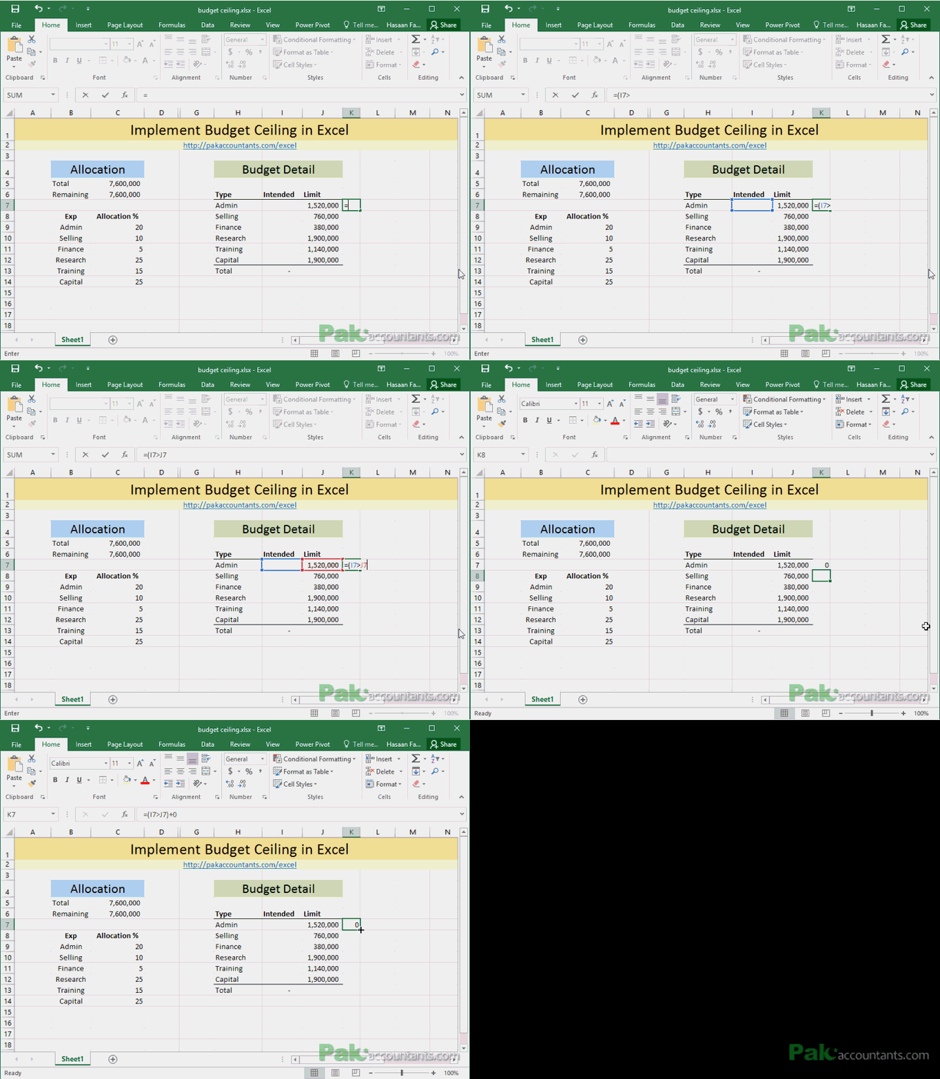
Step 3: Go to cell K7 and put this formula and later drag the fill handle down to cell K12:

=(I7>J7)+0

Step 4: Select cell K7 through K12 and go to Home tab > Styles group > click Conditional Formatting drop down button and click New rules.

Step 5: From format style select Icon sets. Check “Show icon only”.

Step 6: From the icons select the sign you like. I went with the red one and make the necessary adjustments from the drop down menus as shown in the illustration below. Be cautious as a mistake here might render the conditional formatting not to work properly. Once done Click OK.

Test if the conditional formatting is working as intended by putting values in the “Intended” Column.

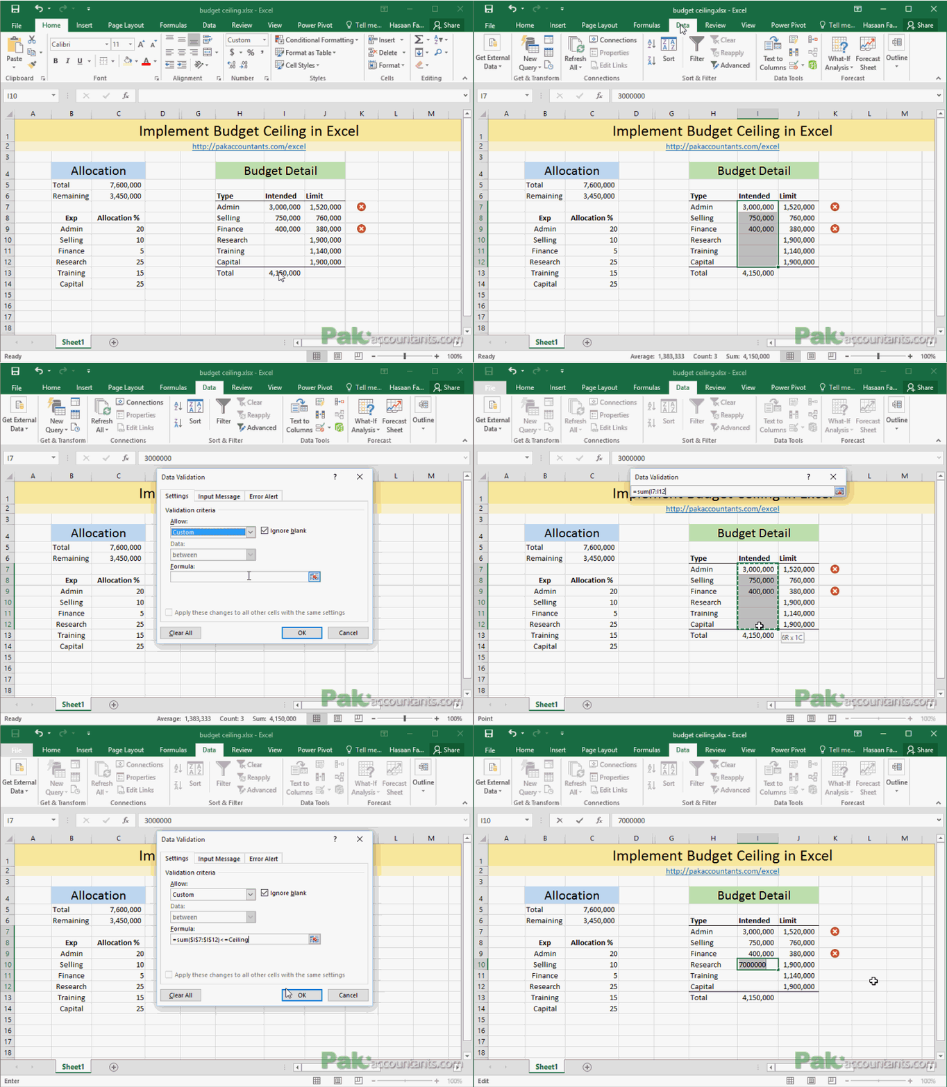
Step 7: Select the coloumn I7 through I12 and go to Data tab > Data tools group > Click data validation button.

Step 8: From Allow drop down select “Custom” and in the formula bar put this formula:

=SUM($I$7:$I$12)<=Ceiling

Step 9: Go to Error alert tab and give the title and message of your desire and click OK. This is the message user will see if the total expenditure exceeds the allowed budget limit.

So you have it! Budget with all sorts of claws and teeth to restrict the darn outflows! 😉