LIFO Stock Valuation in Excel - Template

 How good is it that we learn to automate cumbersome calculations in Excel like FIFO and LIFO. Last time we discussed FIFO valuation using Excel data tables and today we are doing LIFO valuation using Excel employing trusty data tables.

[click_to_tweet tweet=”LIFO inventory valuation in Excel using Data tables – How To https://pakaccountants.com/lifo-inventory-costing-valuation-excel-data-tables/ – Tired of doing LIFO calculation? Not sure how to do it in Excel either? This tutorial is for you with detailed steps and walkthrough to learn swiftly! Join YT channel: https://t.co/JkVyzIoujP” quote=”Tell others! Doing LIFO calculation using Excel Data Tables is now EASY!” theme=”style3″]

LIFO short for Last in First Out method is one of the popular cost flow assumption for inventory valuation techniques. Although its phasing out of many countries as accountants converge globally on IFRSs, still there are industries where LIFO is permitted and will probably stay permitted for fairer financial information presentation.

To learn few more inventory valuation methods have a quick look at this: What are different inventory valuation methods?. To learn about inventory and valuation techniques in detail head over to this free online financial accounting course: Inventory

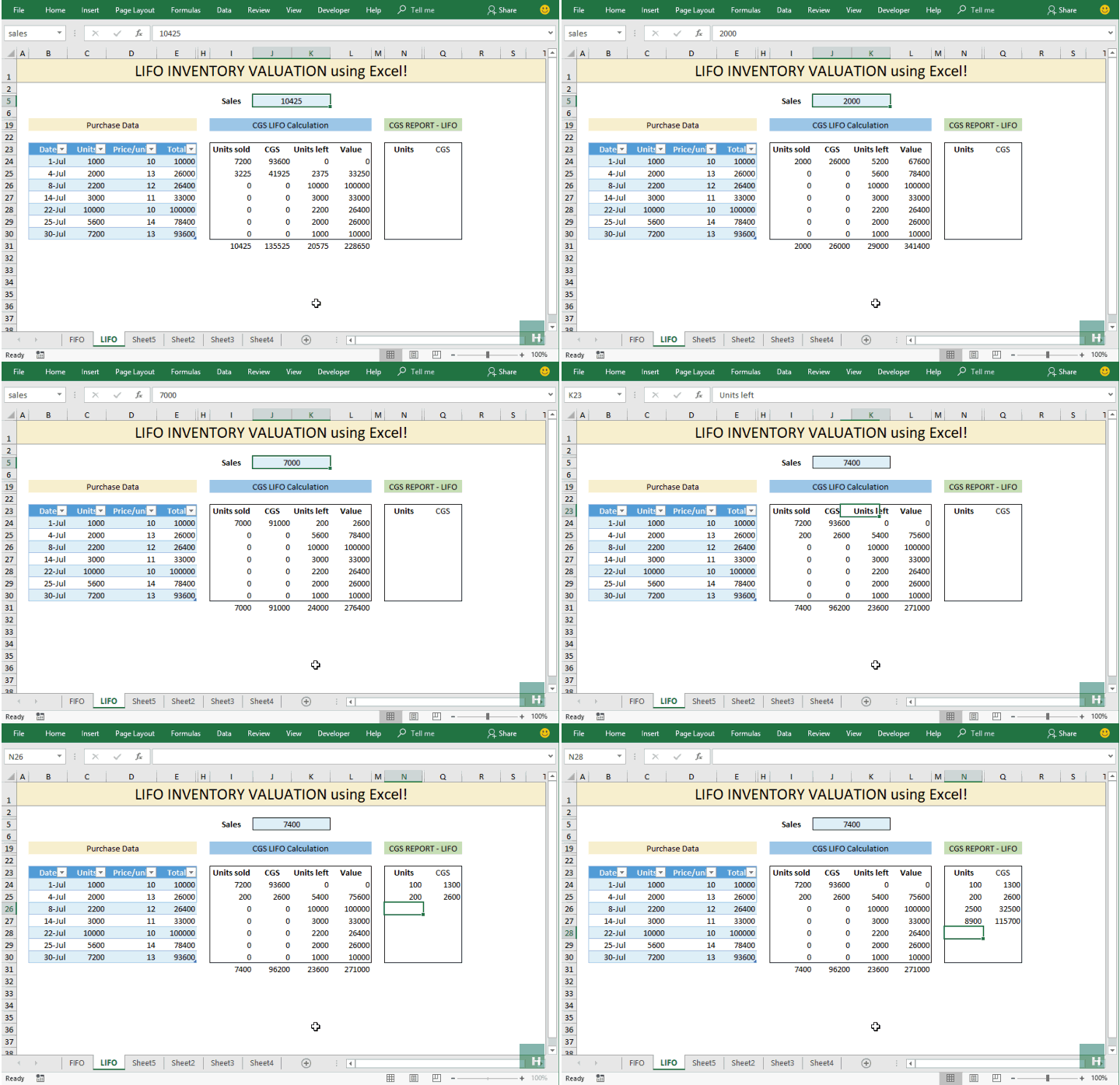
By the end of this tutorial we will have working LIFO calculator as following:

Remember: Excel data tables and Excel tables are two very different features and must not be confused together. Although we will be using both data tables and tables in this tutorial.

LIFO calculation in Excel – Step by step

Step 1: Download this excel workbook to practice the steps of this tutorial to learn along.

We already have the units purchased data. As we are using LIFO for our inventory valuation, every successive issue or sale of units will consist of latest units, i.e. we will start from units bought on July 30th and backwards. For this easiest way is to flip the units and their rates upside down.

Step 2: Units purchased data is already in tabular form and table is named “Inv”. Have an active cell with the total column and give it a name LIFO units. This will insert a new column automatically and put the following formula in the first cell. It will populate itself automatically.

=INDEX(Inv,ROWS(B9:$B$15),2)

Simple INDEX function fetching the value using row number (that is generated using ROWS function) from second column of Inv data range. Data range has seven rows. As we move down the table, row number reduces and thus the order in which value is being fetched is like 7, 6, 5, 4, 3, 2, 1.

Step 3: Use the same technique to get rates by adding another column and pasting the following formula:

Step 4: Name the cell that contains sales amount as “lifosales”. Select the cell containing sales amount and head over to name box. Type in the name and hit enter.

Step 5: Next step is to make a calculator for ourselves and also for report generator that we will mainly use. Go to cell I9 and put the following formula in it:

=MIN(Inv[@[LIFO Units]],lifosales-SUM(I8:$I$8))

In simple word this formula is checking if any unit remains in the latest batch, if not then take the excess units from the next batch. Drag the fill handle down to I15.

Step 6: Now that we have units, we can calculate the remaining respective columns by putting following formulas in respective cells:

In cell J9: =I9*Inv[@[LIFO Rate]]

In cell K9: =Inv[@[LIFO Units]]-I9

In cell L9: =K9*Inv[@[LIFO Rate]]

Select cell J9 till L9 and drag the fill handle down to row 15.

Now to the report, the main objective of this tutorial so that we can calculate the value of units as and when we want for any number of units in any order. The calculator we made helped us give value for one figure of sales. For multiple figures, lets make the solution.

Step 7: Select the data range I9:L16 and press ALT+= to sum the values.

Step 8: Go to cell O9 and put the following formula and later drag the fill handle down to O15:

=SUM(O9:$O$9)

Step 9: Go to cell P8 and refer it to cell containing CGS total under LIFO calculator. In our case it is J16.

Step 9: Select range O8:P15 and go to Data tab > Forecast group > click what-if analysis button and select data table. A dialogue box will open, have the cursor in column input value and select cell containing sales figure > Click OK

Step 10: Put the following formula in respective cells:

In Q9: =P9

In Q10: P10-SUM(Q10:$Q$10) > drag the fill handle down.

Now you can enter any number in units column and it will calculate the exact cost of sales amount for you in LIFO basis.

Step 11: To make the report cleaner, use custom number formatting to hide “0” result. Select the range > press CTRL+1, and in the input bar mention 0;0; > Press OK.

Step 12: Hide the unnecessary bits.

Now you can calculate the cost of sales for any number of units in the report instantly:

Liked the post? Pin it!