Gantt Chart in Excel – How To + Free Template + Online Gantt Chart Creator

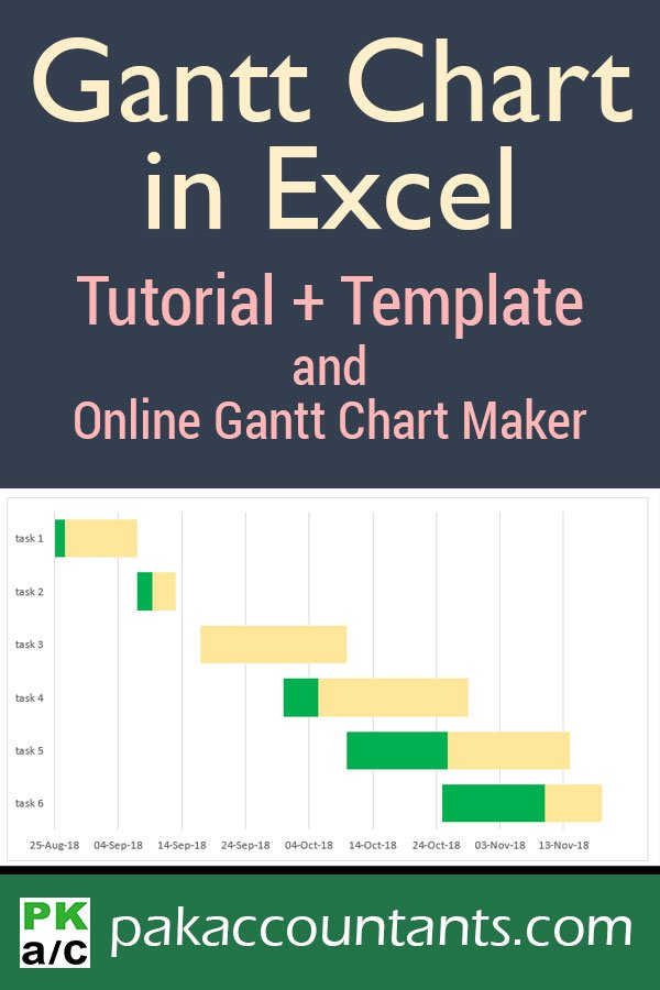
Gantt chart is the simplest-most effective visual for planners and project managers. The most favourite tool to make gantt charts is Excel for two reasons:

1. we curate data in Excel and;
2. Excel stacked bar charts help us create gantt charts easily right inside Excel.

Once made, we can share the files with others as templates. And they can add/delete tasks or make the gantt charts from scratch.

This gantt chart tutorial will explain step-by-step how to make:

1. simple gantt charts quickly using stacked bar chart
2. add completion status in gantt charts for each task by tweaking excel charts with secondary axis
3. dynamic gantt charts using Excel tables so that one can add/subtract project tasks on the fly easily with timeline updated automatically

And also you will have an online gantt chart maker and free downloadable gantt chart template file at the end of this tutorial!

But first lets understand what gantt chart means?

What is gantt chart?

Gantt chart is a graphical representation of project tasks against time in which activities are represented with horizontal lines or bars on the vertical axis or y-axis and time along horizontal or x-axis.

Project is divided in definable tasks and each task is drawn in a separate line over the other wherthe e width of the line/bar shows the duration othe f task and its completion status. Longer the duration, wider the task appears on graph/chart.

Usually a vertical-dashed-line runs from top to bottom showing the current date to give better time-work perspective for viewers’ understanding.

Create a gantt chart in Excel – Step by step

Download this practice workbook that contains the base data for this gantt chart tutorial. It will have you understand the steps taken and practice along to create your own gantt chart in Excel.

Step 1: The file you downloaded contains the project activities, days required for each task and stage of completion.

Have an active cell inside the data range hit CTRL+A to select the entire range of data and then hit CTRL+T to convert data into an Excel table.

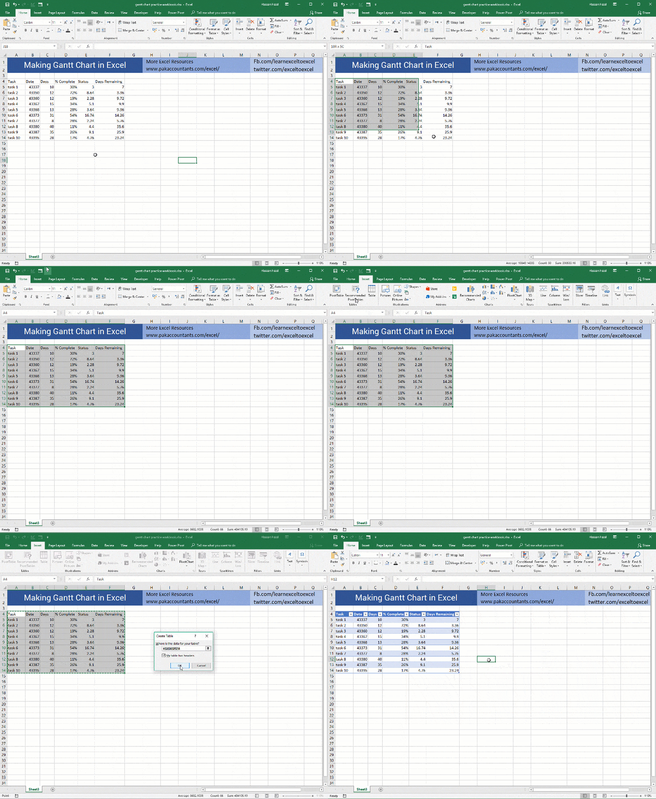
Step 2: You can see that dates are formatted as numbers or “general” number format. I kept this number format so that Excel easily makes the gantt chart as expected and doesn’t plot dates along y-axis.

Hold down CTRL key and select “Task”and “Date” column and while holding CTRL key down, select “Status” and “Days remaining” column and then go to Insert tab > and in charts group click bar chart button and click stacked bar charts. Remember to include the headers in your selection as well.

You can see our gantt chart taking shape. We are almost done, what remains is a few bits here and there.

Step 3: Go to the date column and select the data then change the number format from general to short date or you can have your own custom format in CTRL+1 dialogue box.

Bonus: You can change the number formatting right in the chart as well. Though changing the number format in data will get reflected in gantt chart, but if you intend to keep the data format intact and change it only in chart, its quite possible.

Double click the date which is horizontal axis bar of the chart, axis formatting bar will open on the right > click on number drop down > and in format code input bar type this: dd-mmm-yy > click add key.

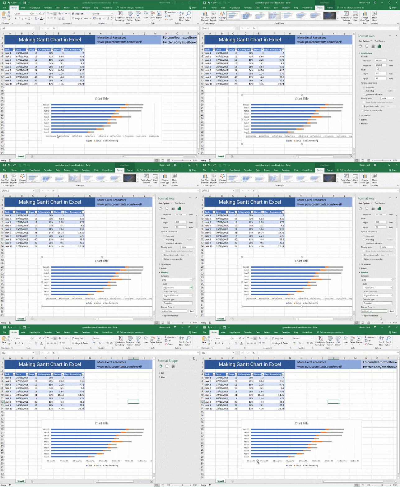
Step 4: Left click once on the first series which in our case is blue and go to format tab > shape fill > click no fill. It will make the series invisible. We don’t need this series and only have it to anchor our tasks at the right data on gantt chart.

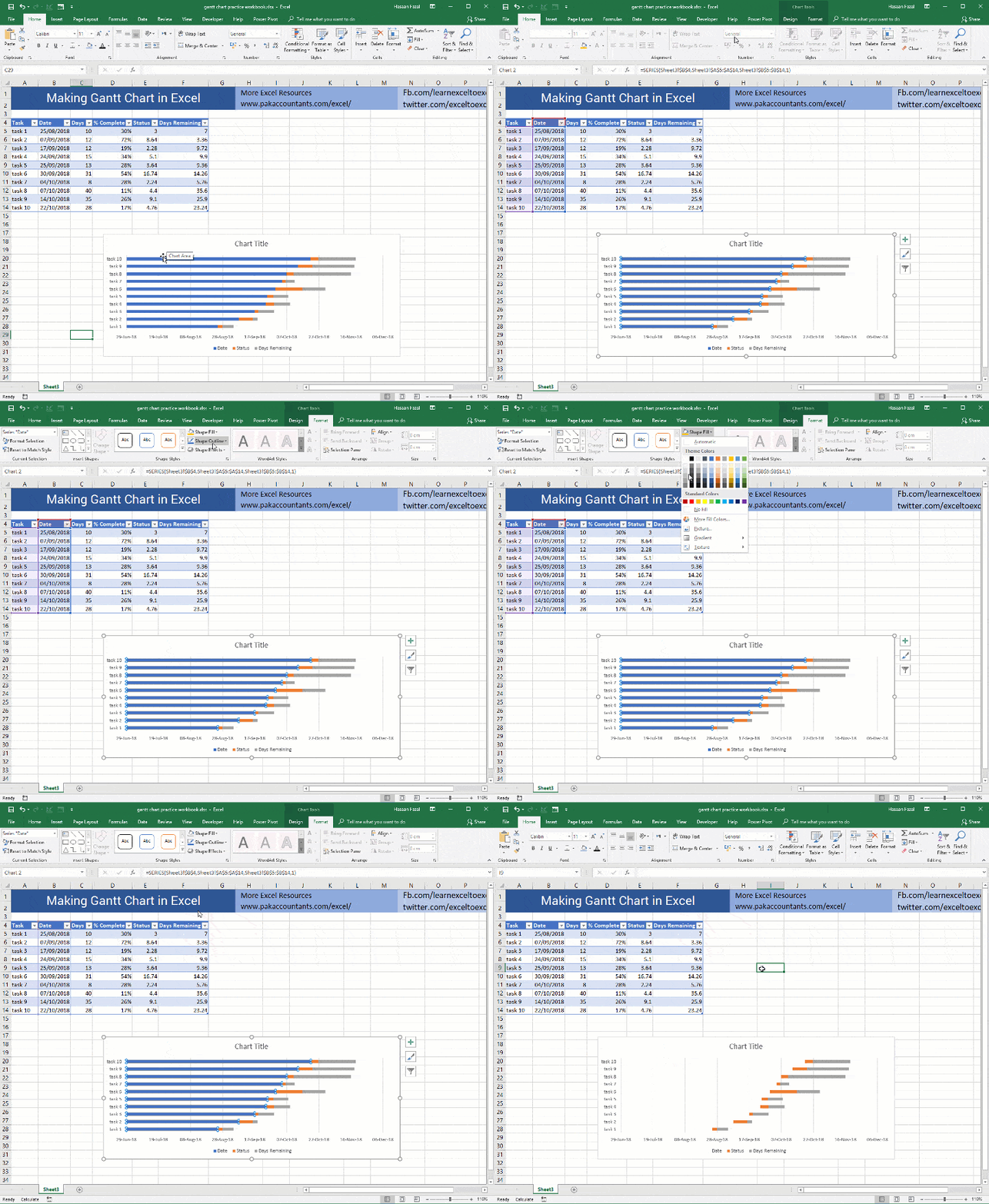
Step 5: We need to adjust task arrangement in ascending order from top to bottom on gantt chart unlike descending order.

Double click on the vertical bar containing task names > Axis option bar will open on the right > Under axis option tab > find check box “categories in reverse order” which is at the last of the tab and check enable it. This will put the project tasks in the right order in our gantt chart.

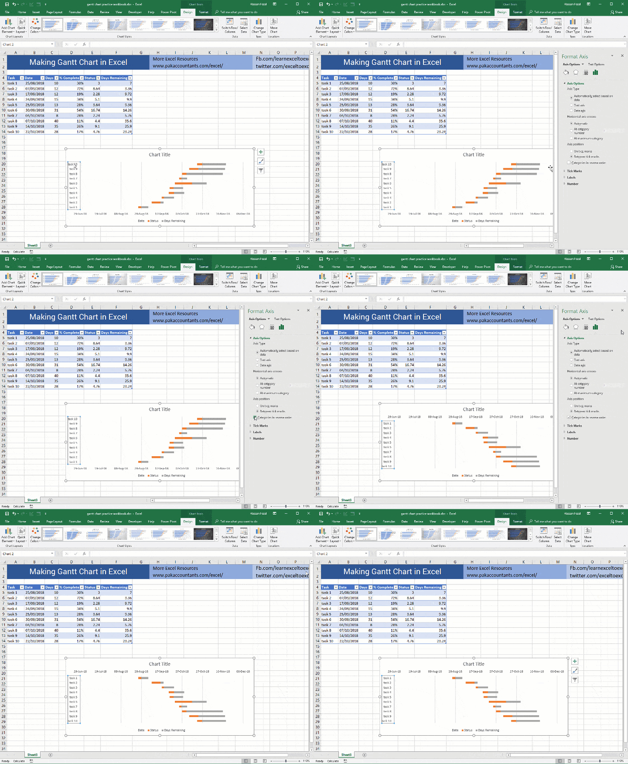
Step 6: Double click on date axis which is at the top after category reversal and set the minimum bound to 43337 which is the number of days for date 25/08/2018. This will bring the first activity at the start of y axis instead of starting in the middle.

To find the number for your date, easiest way is to convert it to general format temporarily and revert back to date format.

Another benefit is activities can be added or subtracted without disturbing the start of gantt chart.

Step 7 : If you wish to keep the date axis at the top then you can skip this step, however if you like to have the date axis at the bottom, then double click on any date > from the format bar at the right click labels tab to open > from position drop down select high.

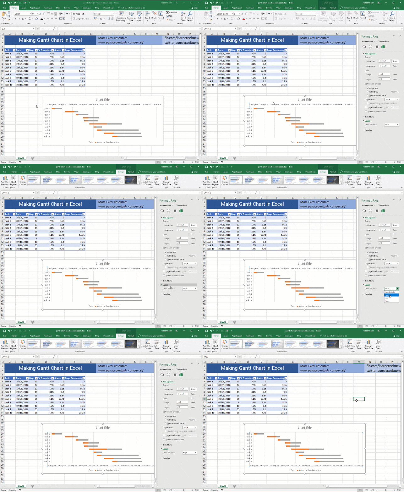
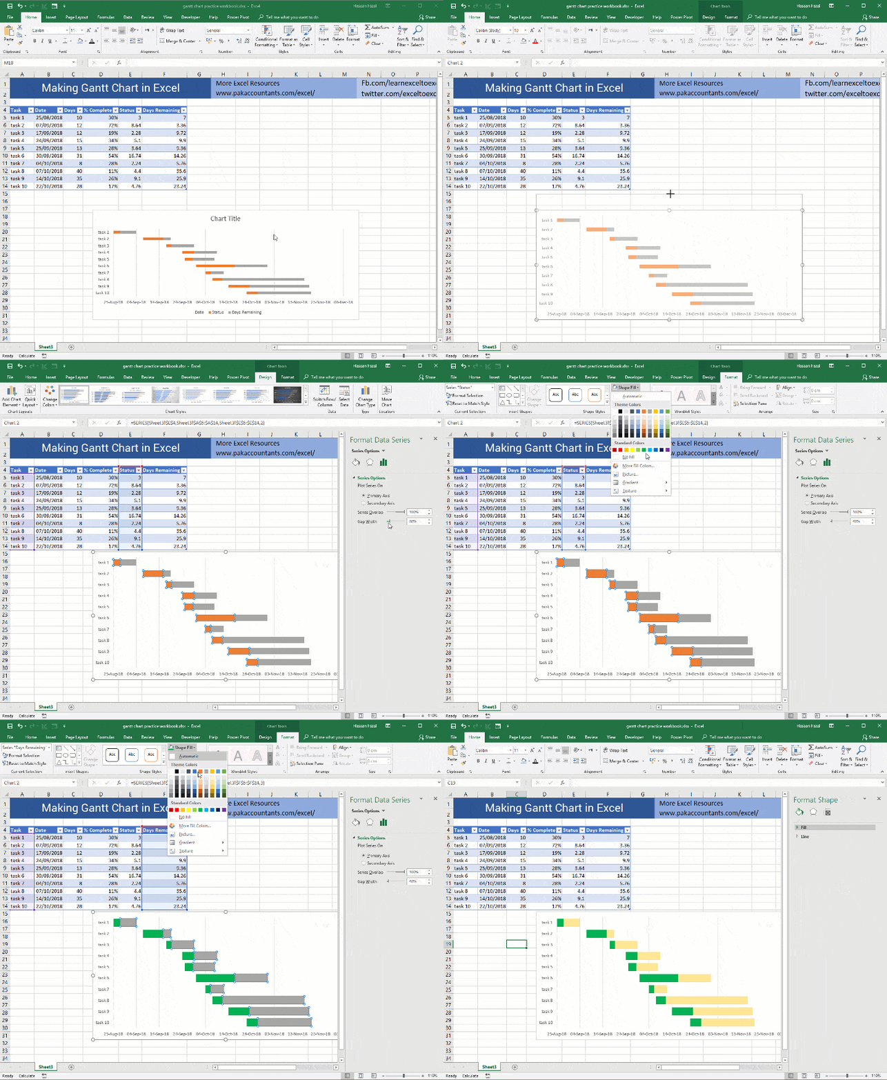
Step 8: Delete the chart title by simply clicking once and pressing delete key. Get rid of legends as well. I have formatted the “% complete” and “days remaining” series as well. Reduced the gap between bars to make them more legible.

Add/Subtract Activities/Tasks from Dynamic Excel Gantt Chart

Now if you like to add another task, its super easy. Simply go to the last cell of the range and hit tab. This will add a row automatically and you can enter the necessary information and gantt chart will update automatically without any hassle!

You can even update your existing activities and their information to reflect in the excel gantt chart immediately.

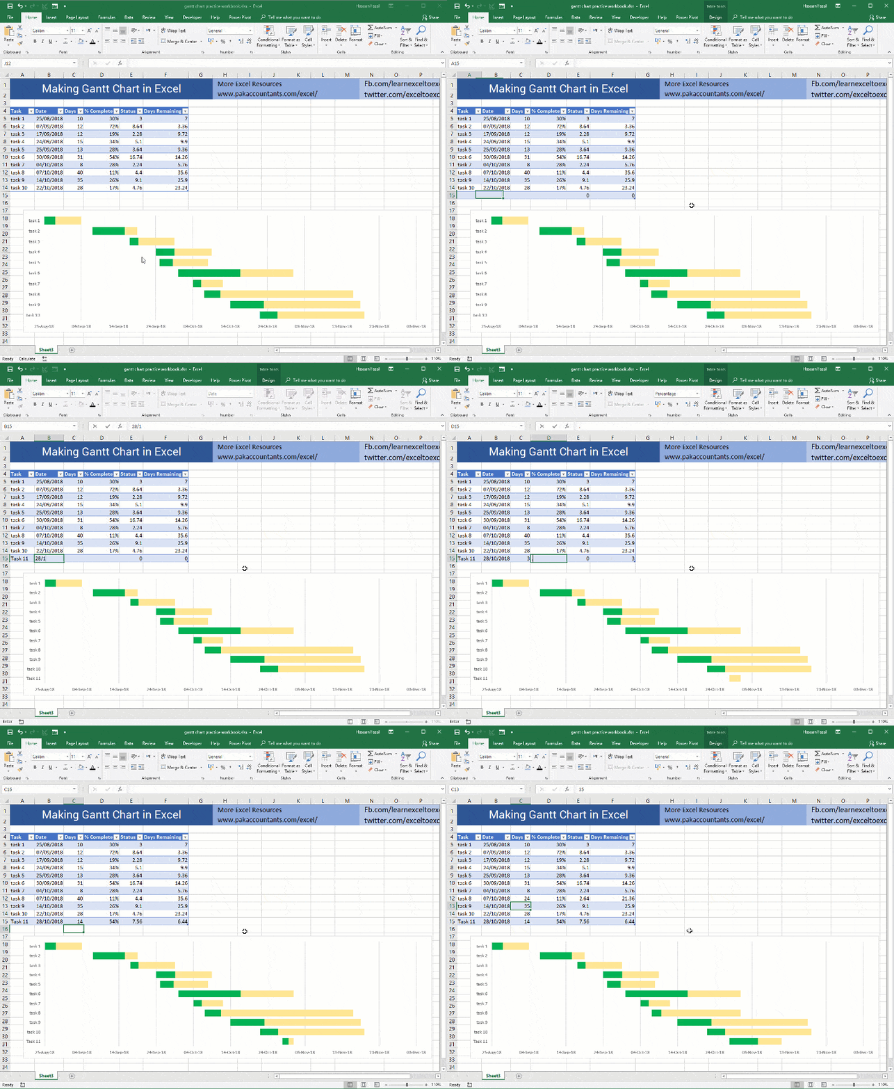
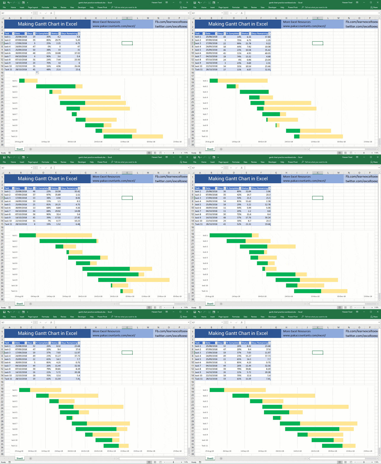
And here is the gantt chart in Excel with random data and see how easily it is updating without any problem! Sweet!

Free Online Gantt Chart Maker

You can make gantt chart online even without Excel installed in your PC. Simply adjust the data as per your requirement and you will have the gantt chart ready for you. And yes you can add, subtract the project tasks as you desire!

Liked the tutorial to make Gantt Chart in Excel? – Pin it!