Excel for Accountants – 10 Must Read Tutorials

Excel and accountants are two interconnected entities. Around the world excel is the most active computer application in the hands of accountants. Even if accountants have some other accounting software at their disposal they always like to involve excel. Most common example is that data entry work is carried out in specialized accounting software but report work is done in Excel.
So we don’t have to emphasize much about the relation of accountants and excel. But surprisingly not much attention has been given in this regard and the work for accountants in excel is still old-school. But it does not mean at all that excel does not have the potential to aid accountant’s work.
Following is the list of hand picked Top 10 Shortcut Keys of Excel to help Accountants in their work. It was a difficult selection and we had to go through each and every shortcut. But after shortlisting several times over, we have come up with these 10 shortcuts which every accountant must know.
10 Select entire table
Select the whole table at once i.e. all the cells (data enclosed in relevant rows and coloumns) within a specific range.
How to use it:
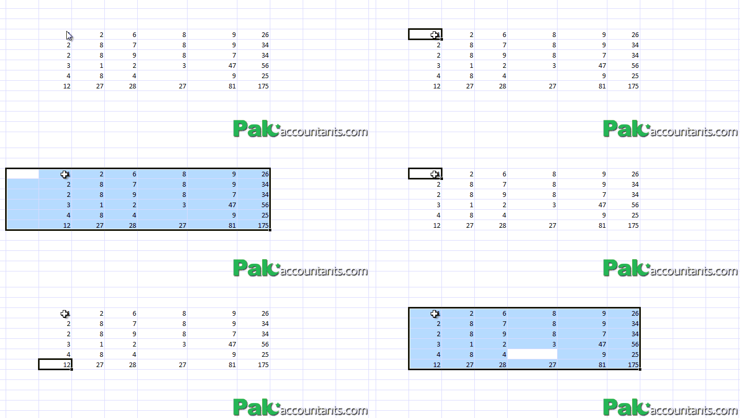
Hold down Ctrl and Shift together and press Space bar to have the selection of the whole table.
Additional notes:
This command however does not work if your active cell is out of range. You must select one of the cells within the range to correctly select the relevant data table.
9 Navigate through different worksheets and workbooks
How handy it would be if you can navigate through different worksheets within one workbook and even jump from one workbook to other without even touching your mouse. You have to do it to be believe it, it saves much time and make work practically efficient.
To switch to next worksheets
To switch to previous worksheets
To navigate through different workbooks
Additional notes:
These navigation shortcuts can work only if you have multiple worksheets and workbooks active or opened.
8 Copy formula from above cell and edit
Think about a situation where you have to copy a formula from a cell and then paste it in the cell just below it and have to edit it. This might seem easier just to say. But in reality its a long cumbersome process which involves multiple key strokes. Just try to imagine the right clicks and double clicks and then right click and then double clicking to do what you want to do.
But what if all this long long process can be done in just TWO key strokes?
How it works:
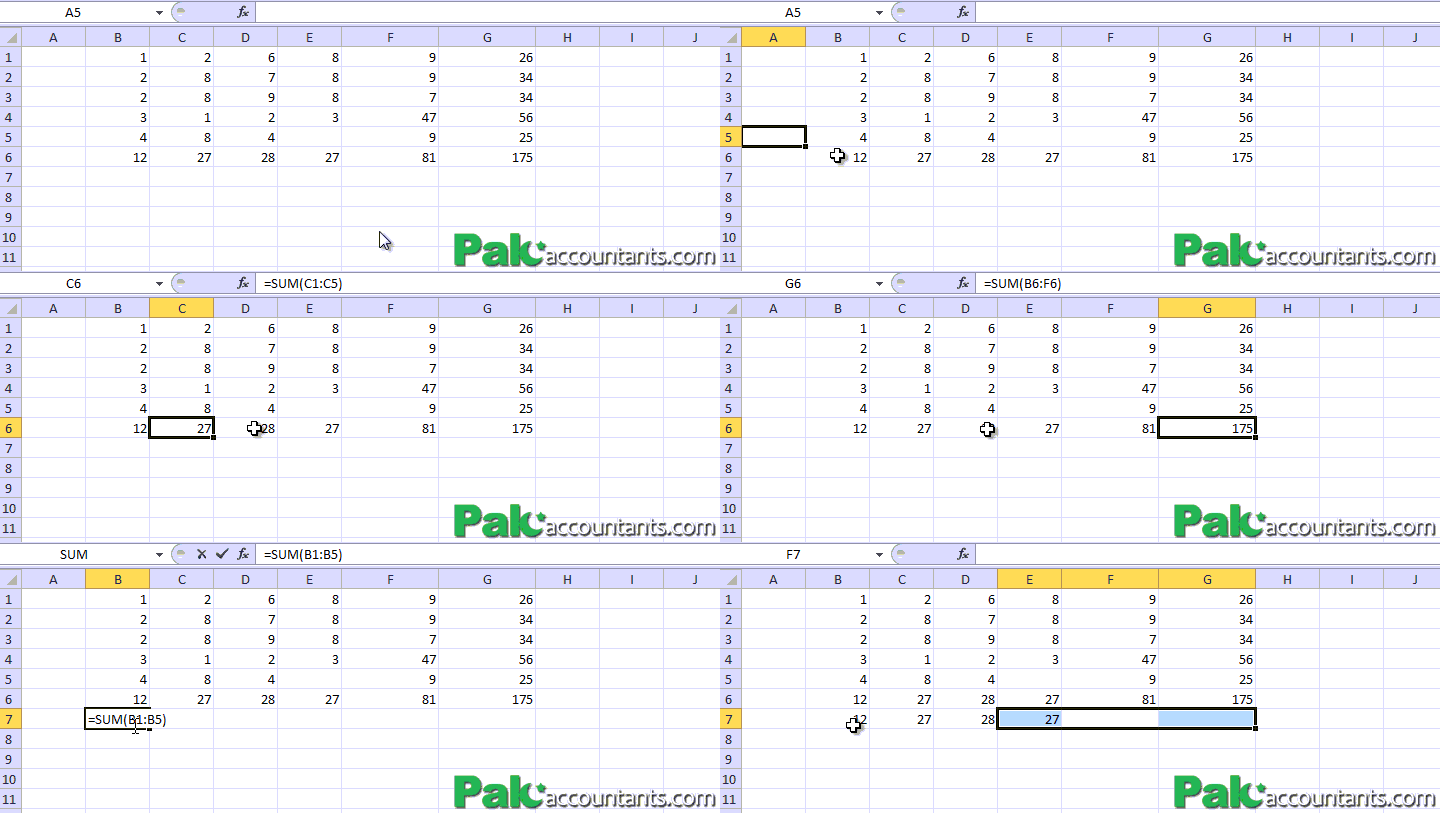
Press and hold control CTRL key and then press apostrophe key. It will paste the formula in the above cell and automatically enters in editing mode thus saved you many clicks and strokes to copy, paste and enter in edit mode.
Additional note:
Before this shortcut can even works as per our desire you need to have:
- A cell that contains the formula we desire and want to edit (mostly minute changes are intended)
- The cell containing formula must be immediately above the cell where we want the modified formula.
If any of the two above conditions are not present we cannot use this technique to its best. Well we should understand one tool cannot fit all needs.
7 Formatting as fast as 1 – 2 – 3 – 4 – 5 – 6 – 7 – 8!
Microsoft is all about all about time saving. Formatting large amounts of data is one big job to execute. But what if we get the help of shortcuts in this area as well.
Number formatting with two decimal places
Format as time
Format as Date
Format as currency value
Format as percentage
Format number in exponential form also known as scientific form
Apply single line border to selection
Make a selection of contiguous cells
6 Detect all cells linked to a formula
What if you are new to a certain data and don’t know what is linked to what. Situation gets more complicated when one cell contains a formula that depends on data in many other cells. Things would become so easy to understand if you are able to know each and ever cell on which a cell is directly or indirectly dependent. Well our next short cut is just for this job!
How it works:
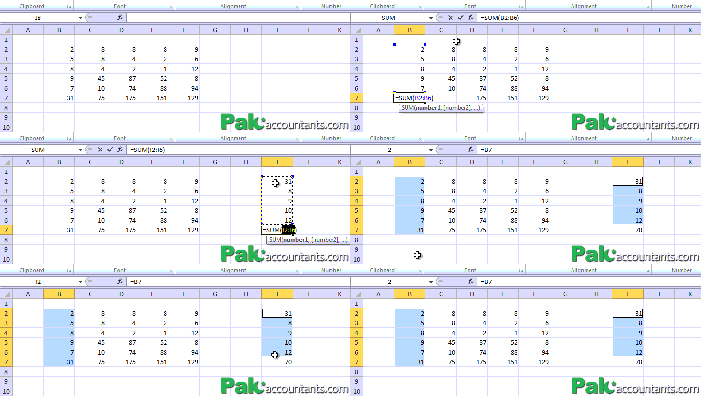
Hold down Ctrl and shift keys together and while pressing hit left braces key and voila! all those cells which help execute a formula will be selected instantly and you can easily get how are you getting what you are getting! Got it?
Additional notes:
Although it would have been tremendously awesome if we had the shortcut to know what cells are depending on a particular cell value or what formula is depending on a particular cell, however, this command only helps you find the opposite i.e. finding cells on which a formula is dependent.
5 Selecting cells quickly and correctly
Ever wanted to select all the cells to the right, left, up or down to the last cell within a specified range? And above that don’t want to reach out to mouse, hold on to left click and drag. Believe it or not, we have a better way to achieve the same.
Ctrl + Shift + Direction keys
How it works:
Hold down Ctrl together with Shift and press the appropriate direction key to select all the cells within relevant range in that direction.

Additional notes:
The major advantage in terms of accuracy is that through this technique selection is made up to the point a blank cell is reached.
4 All existing values in a drop down list! – An auto complete list
During a busy data entry day one would be happy over the moon if excel starts entering data automatically or at least some part of this hectic job is automated. If you are thinking of usual auto complete feature that appears in the cell while typing can be of help to certain extent but most of the time it is annoying. But this is not the only auto complete feature excel offers. What if all the data entered in the same coloumn above appears before you in a list from which you can select precisely? Well it is very possible!
How it works:
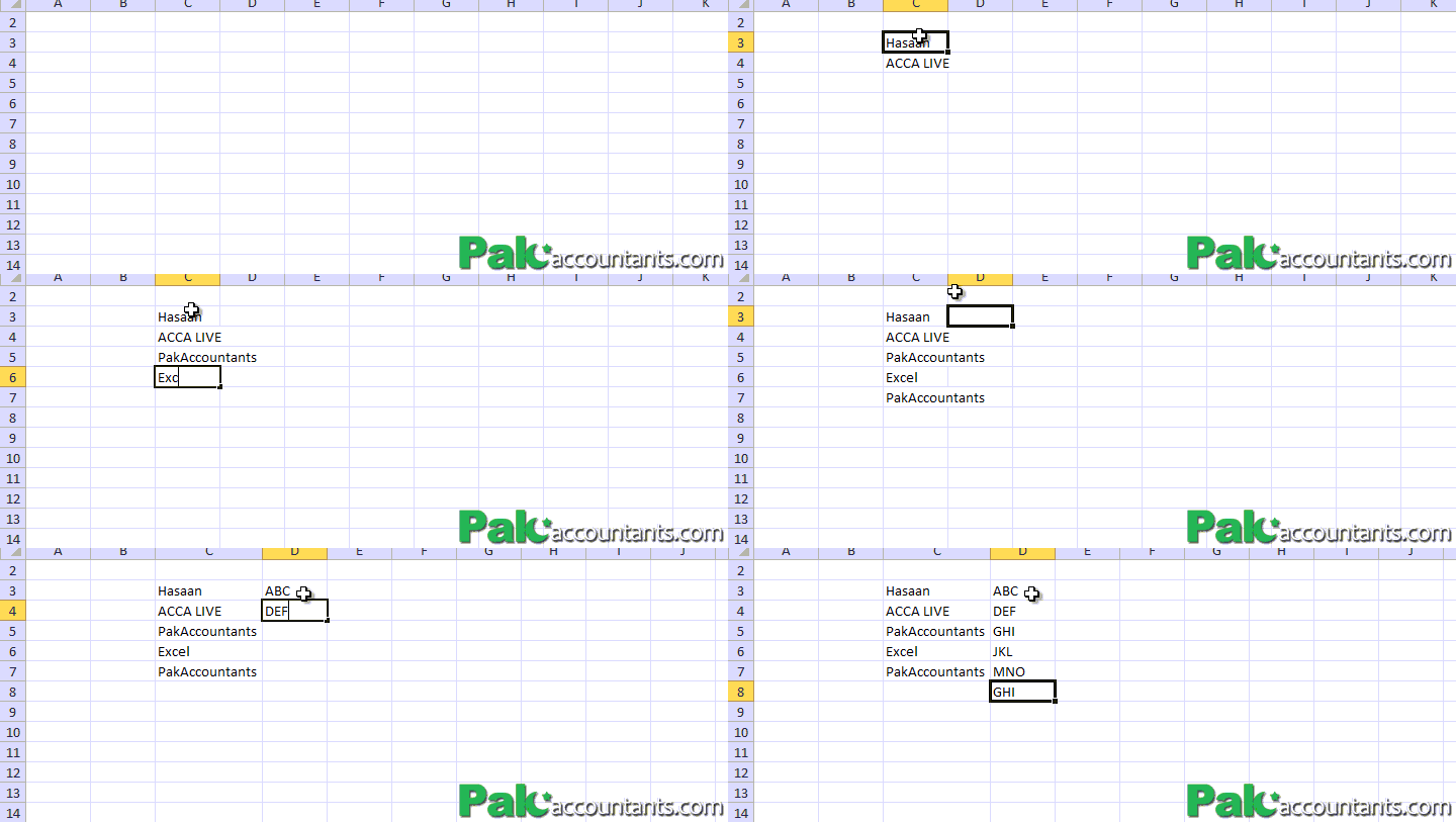
Press Alt with down arrow key and bingo! you have the list of all the values entered so far in the coloumn. And this is not an ordinary list. It comes alphabetically ordered.
Additional notes:
It might not be as reliable as it is thought to be. Sometime items are listed and sometime not. And if a data has blank cells in it, then it would be even more unpredictable and disjointed. One of the key benefit of this shortcut is that you can use this feature above the range or below the relevant range. Unlike autosum function, you don’t have to be always at the bottom of the range to execute the command. However, one limitation is that the list will be display only that data which is entered in the same coloumn in which active cell is where you applied this shortcut. For example the content entered in coloumn B will not be available in the “auto complete list” if the combination is applied in any cell of coloumn C or any other coloumn except B. So you have to be in the same coloumn where your desired data is to have it in the pick from the list drop down selection.
3 Toggle between cell value and formula
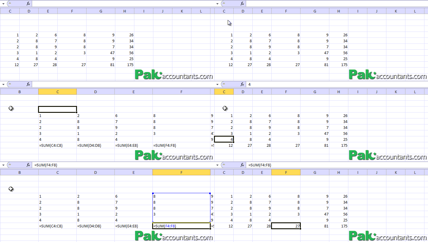
This shortcut is the evidence that power does not always come without convenience. Usually excel users have to double click the cell to view the formula and that only reveals formula in just one cell. The next shortcut in our top ten list reveals the formula across the excel worksheet.
How to use it:
Press and hold Ctrl key and then press Tilde (back quote).
2 Selection again – Extended selection
This is one of those lesser known gems of excel. If you want to make a clean, smooth selection of cells but without using mouse, you can make as big selections as you like with our next shortcut which is one short to be our king of list.
How to use it:
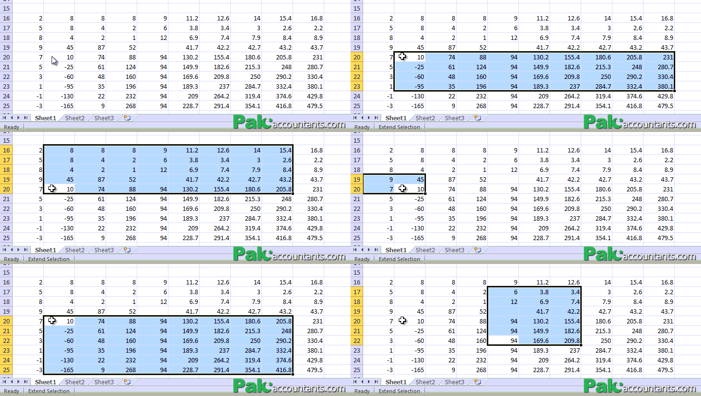
Press F8 once and use direction keys to move the selection in the appropriate direction to select desired cells. You don’t have to hold down “Shift” key to do the selection. Once F8 is pressed and ‘Extend Selection” mode is active you can either use direction keys to make the selection or mouse to make or extend the selection.
Additional notes:
Once F8 is pressed a notification of ‘Extend Selection’ can be seen in the bottom status bar of excel to let user know that extended selection mode is enabled. Pressing F8 again will disable ‘Extend Selection’ mode.
1 F4 – Toggle cell reference / repeat last action
One of my personal favourite and no doubt king of keys. Many people know this key probably for one reason. But this key has one more function up its sleeve which is not known to many. This one very function key can do wonders in the way you structure and populate your excel sheet. I have to admit, this very key deserves respect and each of the two uses must be explained at full length separately.
Toggle absolute and relative reference
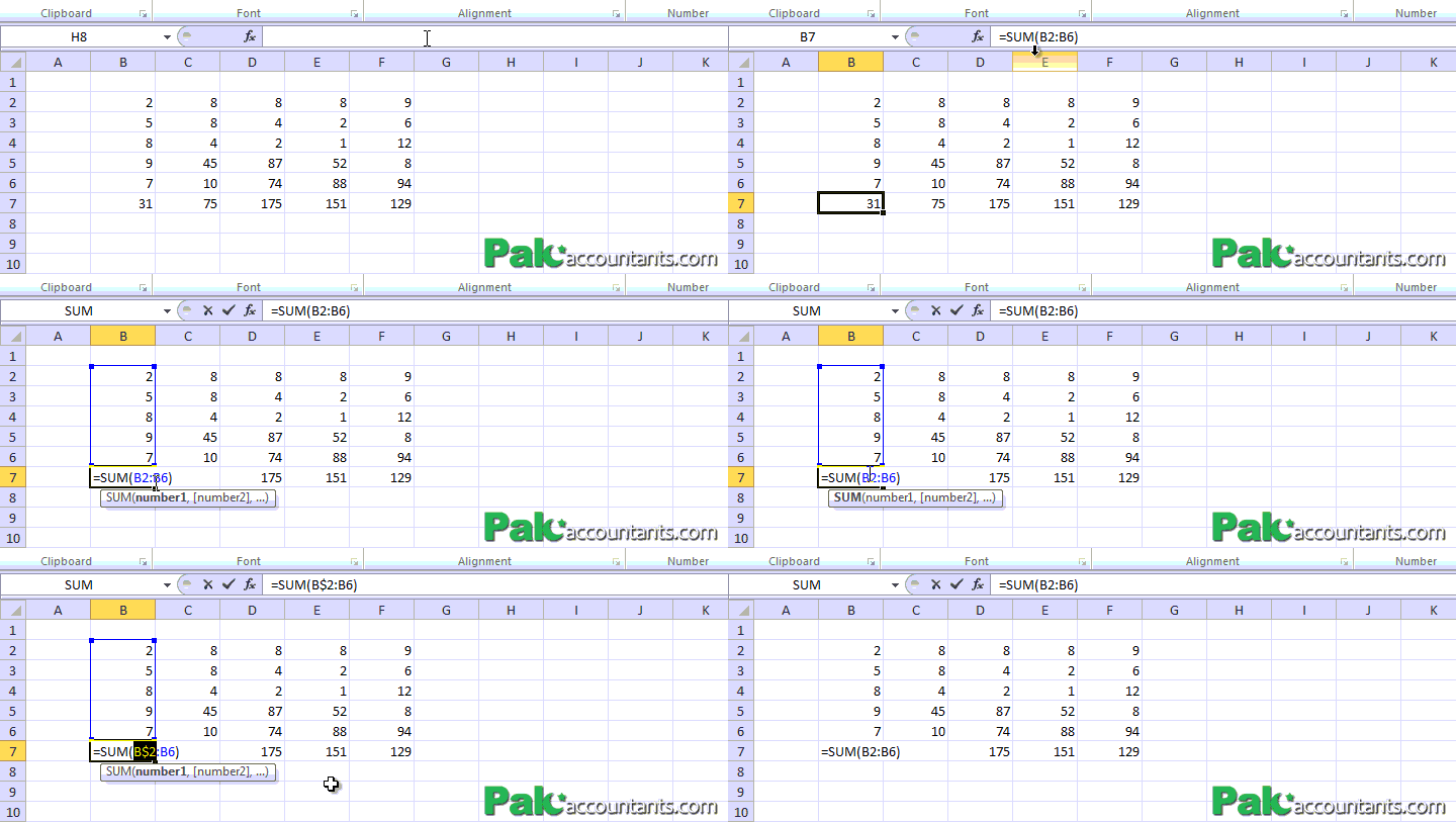
With formula in edit mode move cursor to any cell address and press F4 key. You will notice dollar sign ‘$’ appearing before row letter and / or coloumn number. There are four different cell referencing options to choose from. Pressing F4 will cycle through these 4 options. So remember, 4 referencing options using F4.
Repeat last command or action
If you are doing something on repetitive basis let it be a formula, pasting, formatting etc then instead of pushing key combination over and over again you can do it just by pressing F4 while in non-editing mode. For example if you have copied a certain value and wants to paste it in several cells then you don’t have to click paste button with mouse or Ctrl + V again and again. Just press F4 and it will be pasted. F4 repeats the last action you did conveniently for you.
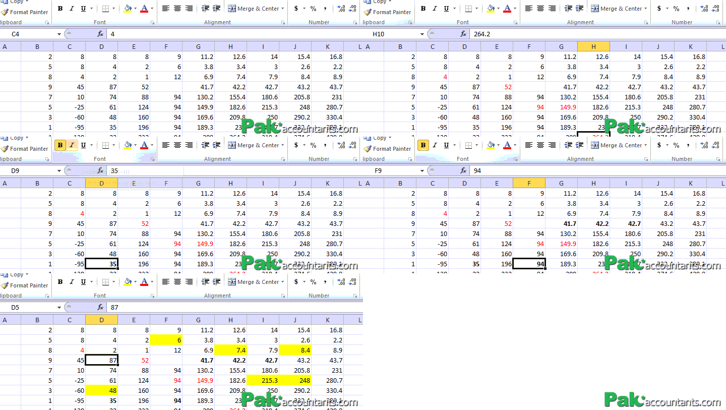
Take another example, you want to underline certain cell values then instead of clicking underline button in home tab or hitting combination of Ctrl + U, just do this once and later only press F4 to underline other values.
Repeat latest activity. This is yet another beauty of this king of keys in excel. And above all it works in other office programs as well.
Bonus keys
Minimizing ribbon
At times you wish you had even bigger screen space while working on excel. In 2007 and later versions “ribbon” concept has been implemented. This ribbon use up quite some precious screen space. But do you know that it can be minimized and maximized when you want it easily using a shortcut?
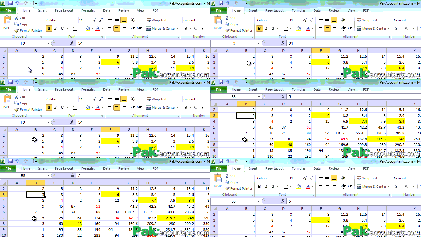
How it works:
Press and hold Ctrl key and then press F1 with it. The ribbon will minimize releasing more screen space to work on excel sheet. However, if it is not working then click the ribbon once and then hit the combo it will work!
Awesome Autosum
The mighty auto sum function of excel needs no introduction. It is probably one of those formula which is learned by everyone who is using excel for the first time.
However, the brainy heads at Microsoft understood correctly that just a dedicated button to insert sum function is not enough. So you have been provided with a shortcut key as well to execute the same auto sum function without looking for auto sum button in the ribbon (or menu if you are still using Office suite older than 2007.)
How it works:
It works in two ways:
- Select the cells first for which you need the sum and extend the selection by one cell i.e. one empty cell at the end where the results will be posted once you hit the combo keys
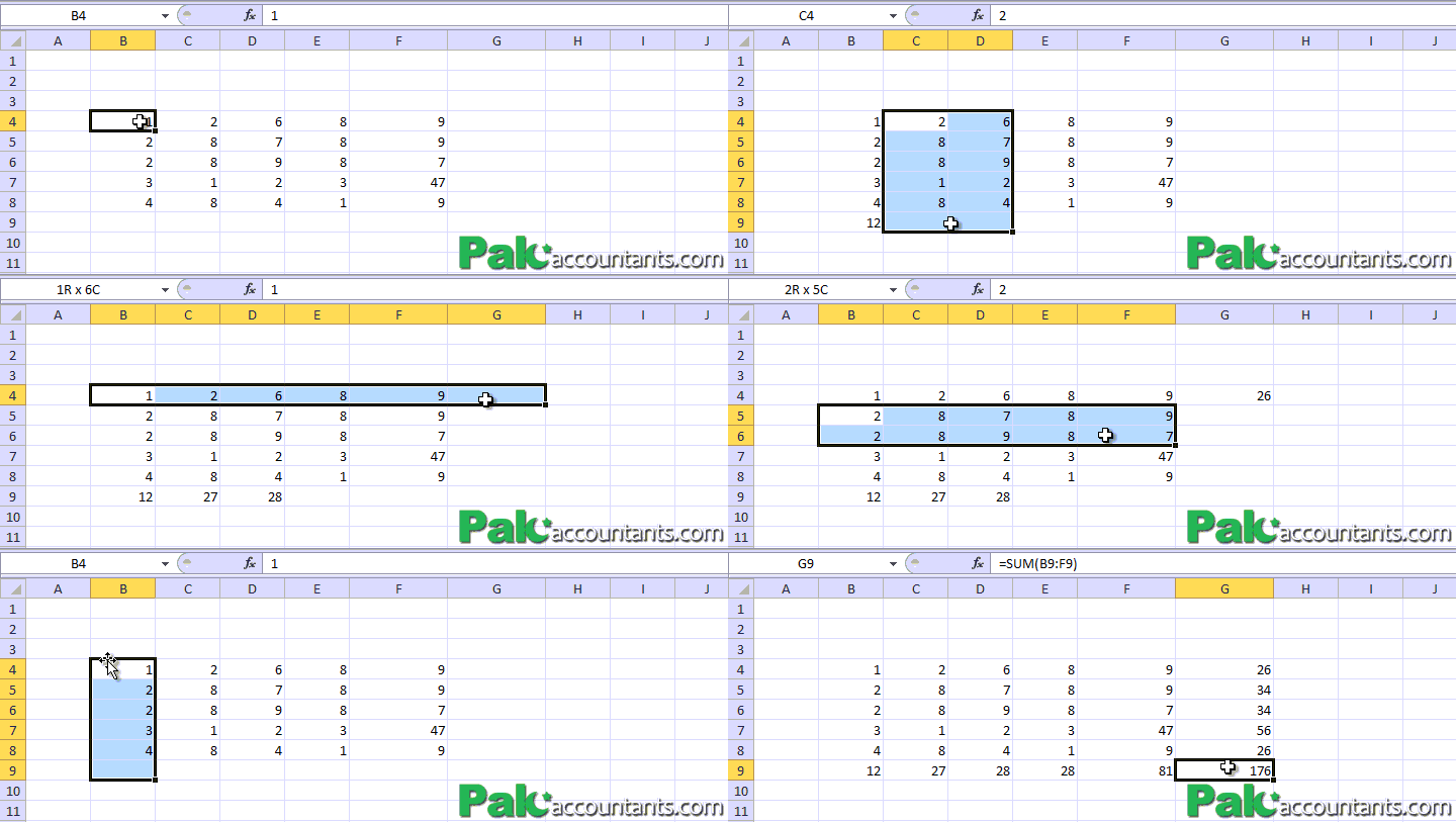
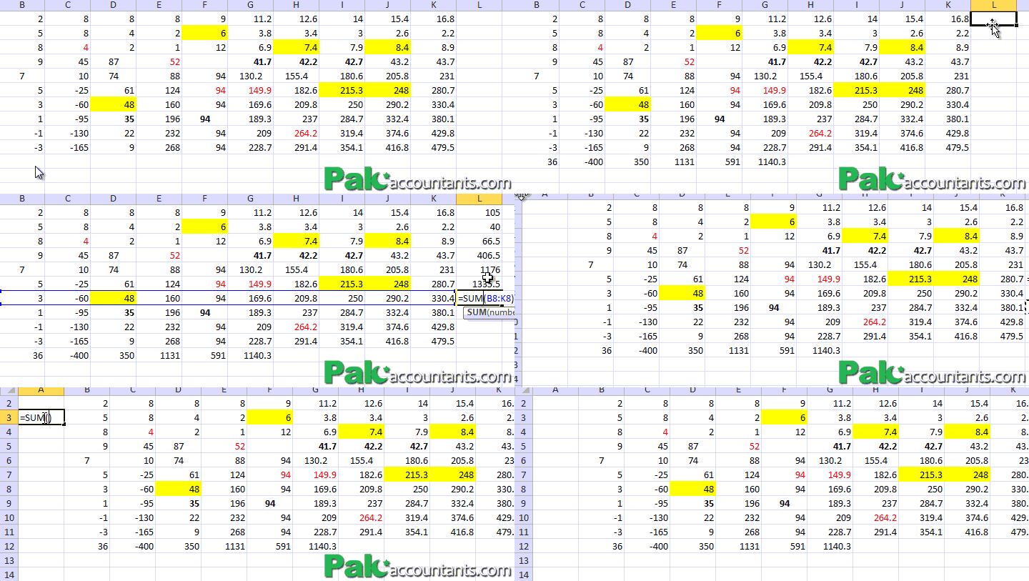
- Simply select the last empty cell of relevant range and hit the combo and it will do the autosum for you by automatically selecting the range at left or above the cell selected. It won’t work if you try to get autosum by selecting the far right cell of the range or the cell which is above or at top of the relevant range.


Leave a Comment