Excel DSUM Function – “The” Sum function you MUST know

You must have learnt SUM in your early days of Excel and later might have learnt about nested IF statements to do conditional sum and you might have already learnt about SUMIF and SUMIFS.

But there are situations when you can have nervous breakdown trying to make a formula. That is why many resort to pivot tables even for one simple sum. But today we will learn one function that to me is as powerful as all these sum functions combined i.e. DSUM.

Here is one situation with different requirements:

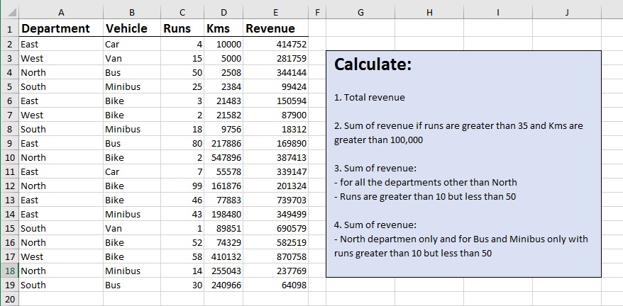
So we have four different situations in which we are asked to calculate revenue. Mind you each bullet under each point is not a separate situation rather conditions that we need to implement.

Few words about DSUM. Here is the function and its syntax:

=DSUM(database,field,criteria)

database: simply put the data range with headers inclusive.

field: in simple words the column we like to SUM. In our case it is revenue

criteria: range of cells where criteria is mentioned.

How DSUM Works

DSUM function is a little different from other functions because it is a database function. D = Database.

Concept of database should not be alien to Excel users, however, databases tend to have different terminologies. For example:

1. For database we use the word data range or table or simply range.
2. Databases have fields whereas in Excel we call them columns.
3. Databases have records whereas in Excel we call them rows.

Understanding how DSUM criteria works

As I mentioned earlier that for DSUM we express the criteria in a range of cells following the same structure as the database itself i.e. we can mention criteria for each field by mentioning it as a header and then giving the criteria under it.

Example 1

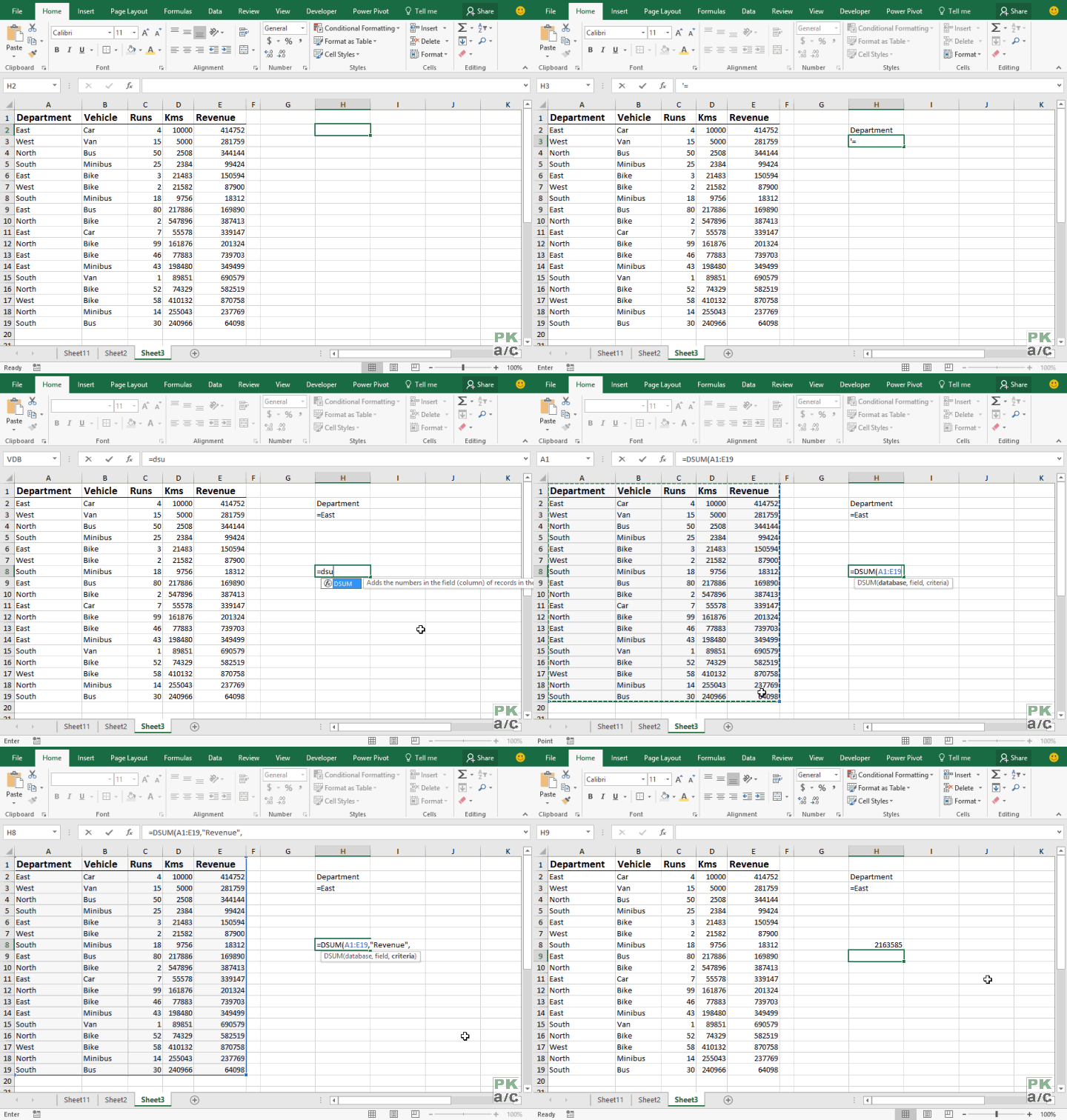
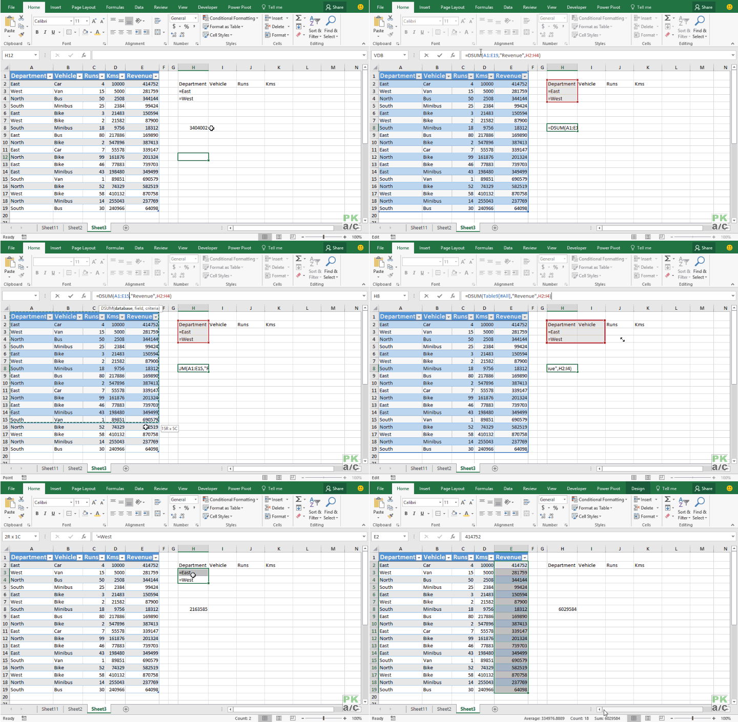
Lets say we want to sum the revenue for east department only. To do this take following steps:

Step 1: Mention the heading which is exactly same as the header in main data range. In our case it is department that I mentioned in cell H2.

Step 2: In cell H3 type: ‘=East. Press Enter.

Notice that I put apostrophe before equal sign. This is to ensure that input is text based. On pressing Enter key you won’t see apostrophe.

Step 3: In cell H8 put this formula:

=DSUM(A1:E19,”Revenue”,H2:H3)

Example 2

Lets say we want to sum revenue for East and West only.

For this we need to make a change in criteria range and also in the formula to accommodate the changed criteria range.

Step 1: In cell H4 type: ‘=West

Step 2: Change the formula in cell H8 as following:

=DSUM(A1:E19,”Revenue”,H2:H4)

You can see that as the criteria range has one additional row, our formula has changed from H2:H3 to H2:H4 to consider the new condition.

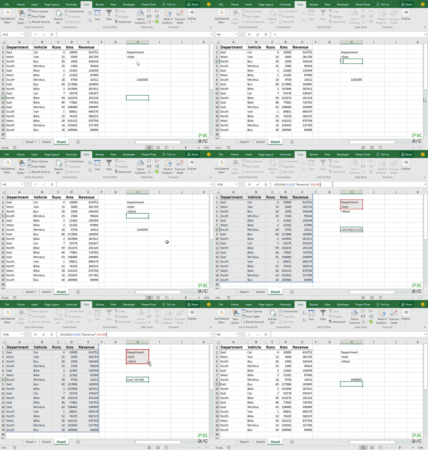
An important point to understand here is that East and West are two separate records and each of them can have additional conditions associated to them independent of each other. I will explain that later with example.

A recap:

1. You have the data range with different fields i.e. departments, Vehicle, Runs, Kms and Revenue.
2. The field that needs to be summed is mentioned. In our case it is Revenue.
3. I mentioned the field name for which I want to apply criteria and then mentioned the criteria under it in text form by appending apostrophe.

Calculating the requirements

Now lets move ahead and get the requirements done. Here is the situation once again:

Setting up the solution

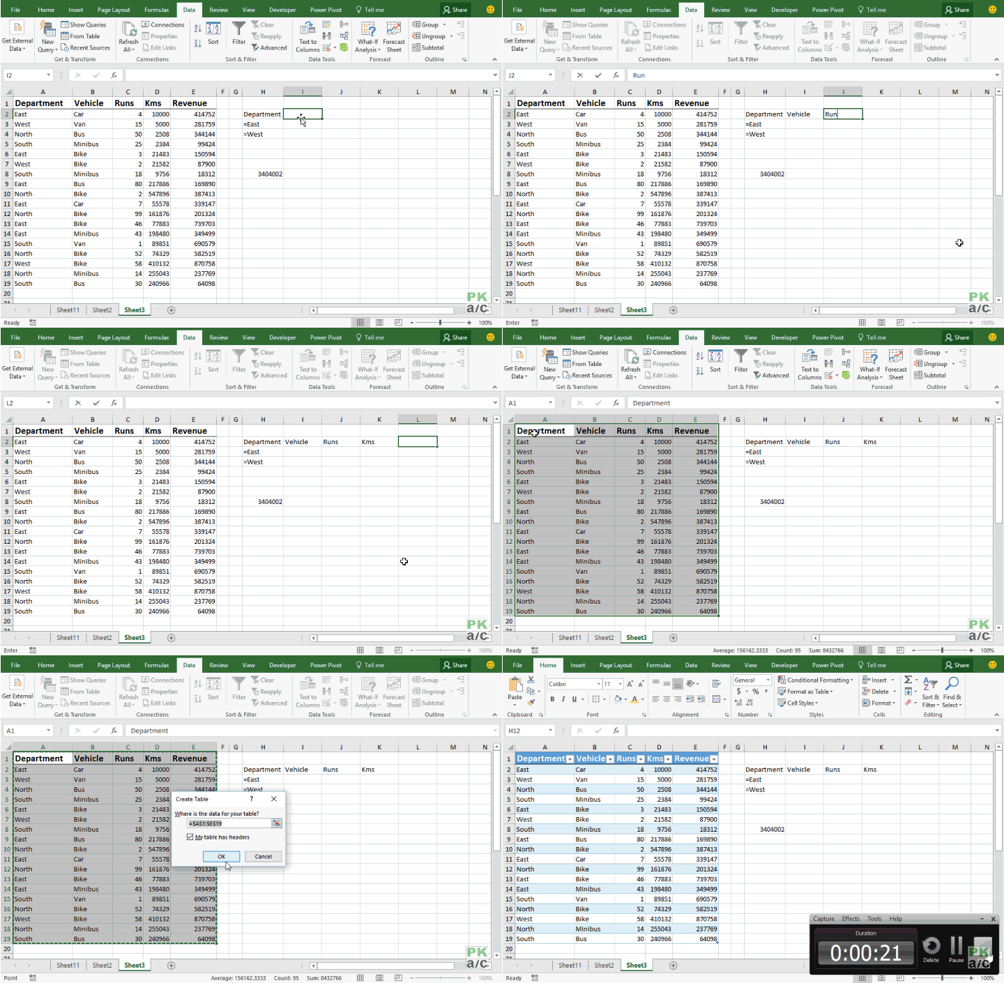
With criteria range already changed to table, add few columns to have all the fields of data range. Currently it has only Department field.

Select the data range hit CTRL+T > make sure “your table has headers” option is checked. This will help make the data range dynamic.

Situation 1

This one is easy. Just delete anything written under criteria fields and result will automatically be sum total of revenue.

Change the formula in cell H8 as following:

=DSUM(data[#All],”Revenue”,H2:L3)

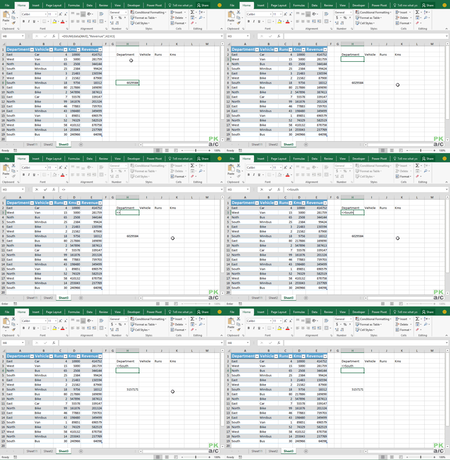
The above formula will give you the total revenue. You can confirm the total by simply selecting the revenue column excluding header and check the info in the status bar below.

Bonus: Summing all excluding few

Suppose we want to sum revenue from all the departments excluding South. For this we need to give criteria under department as: ‘<>South.

“<>” simply means ‘not equal to’. With no change in formula needed since Situation 1 following illustration shows the process:

Situation 2 

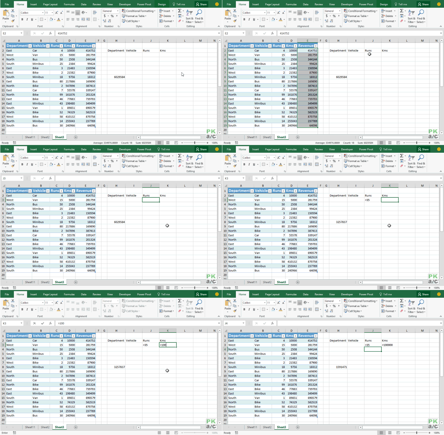
In this situation we have criteria only for “Runs” and “Kms” fields which you need to enter as following:

For Runs: ‘>35
For Kms: ‘>100000

Important: Make sure that there is only one row in criteria range otherwise it will not work. The reason is if you have one row with criteria and second one empty, the empty row will nullify the conditions in first row thus what you will see is the same total revenue figure as in situation 1.

Situation 3

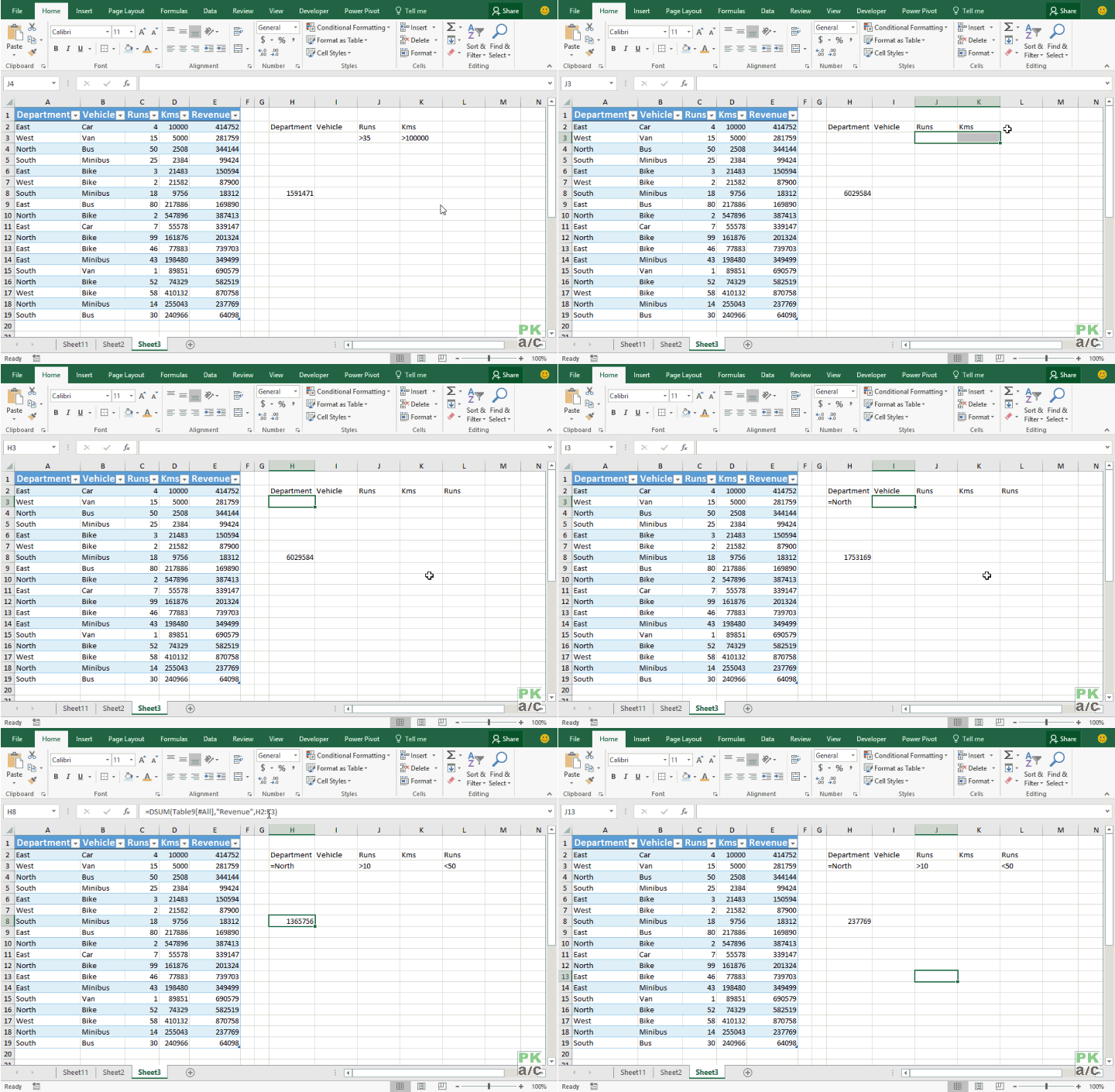
In this situation we need sum of revenue from all the departments excluding “North”. But has a twist for “Runs” that are required to be greater than 10 but less than 50.

We already have one field for “Runs” in criteria range where we can mention greater than 10 but to mention less than 50 we will have to add another field with same header i.e. “Runs”.

Under first Runs field put: ‘>10
Under second Runs field put: ‘<50

Change the formula as following:

=DSUM(data[#All],”Revenue”,H2:M3)

Situation 4

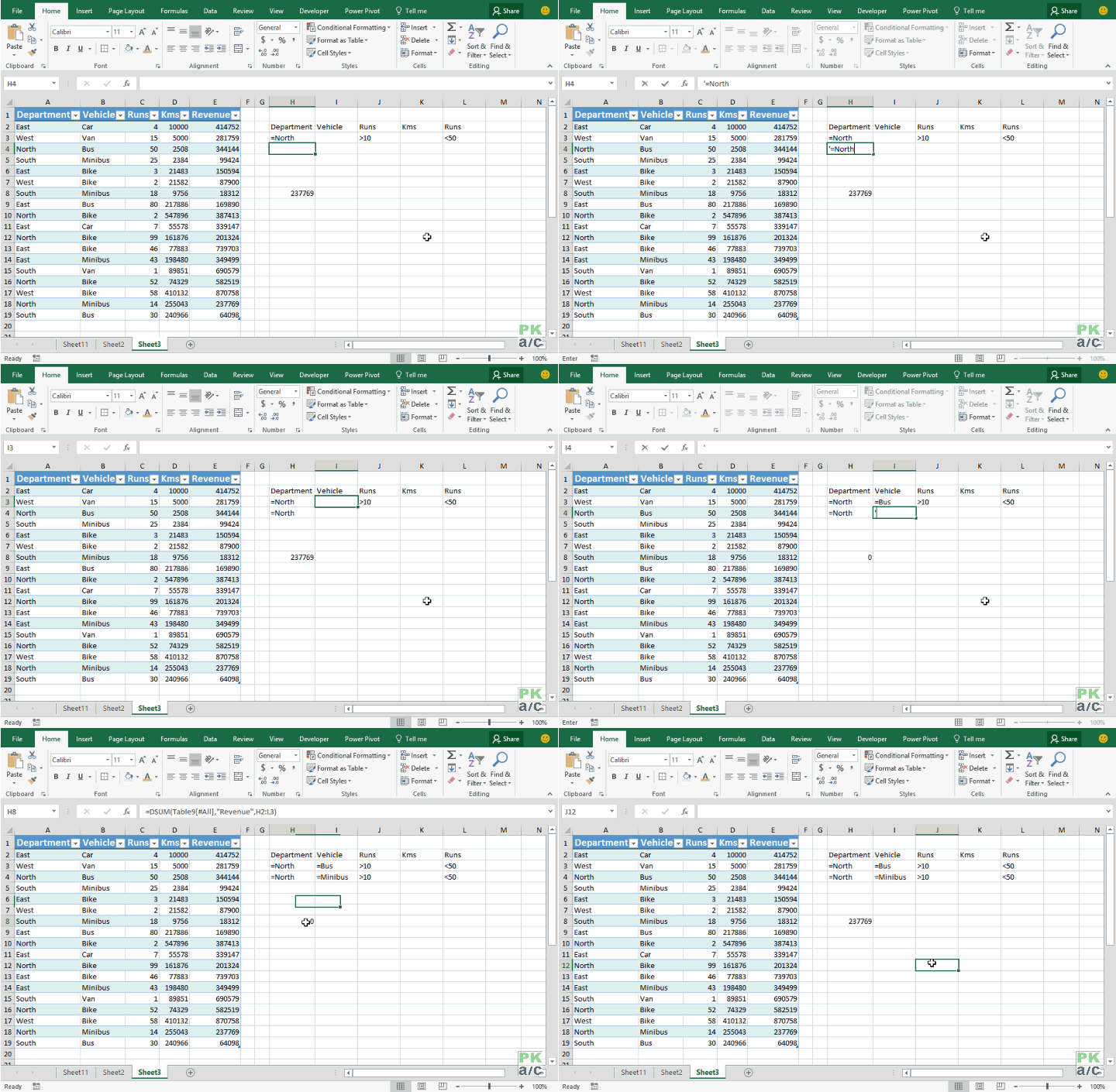
In this situation we want to take sum of North department but for only Bus and Minibus. And also with runs greater than 10 but less than 50. Both of these will be added in two separate rows as following with a slight change in formula as well:

Challenge!

Now that we have seen several examples on how DSUM can help us SUM data with different criteria, lets take it up a notch and see if it can still hold itself together.

Taking the same example as Situation 4 but with one additional condition that we want to include the revenue from other departments as well excluding bike.

So situation should probably be read like this: “Sum revenue from all departments excluding bike but for north include only bus and minibus”.

Suggest your criteria design in the comments and lets get the discussion started!