These Pivot Table tricks massively save your time

These Pivot Table tricks massively save your time

Pivot tables are powerful. Use these 6 tricks to save time when working with them.

New to Pivot Tables? Check out this introAre you new to Pivot Tables or just used them a few times? Then check out this excellent getting started with Pivot Tables guide.

1 - Double click to see details

Ever wondered what numbers add up to the total in a pivot table value area? Simply double click to investigate. Excel will show all underlying values. 

Extra tip: Don’t forget to delete such detail worksheets as they can create duplicate data.

2 - Format value fields quickly

The default value field formatting is useless. Often, we need to change the values to currency or accounting formats. You can do this quickly by right clicking on the values instead of going to Value Field Settings > Number Formats route.

See this image to understand the process.

3 - Include filtered items in subtotals

Let’s say you have a pivot table with Sales by product & region. You filter out some products. The grand totals change. This can be inaccurate.

If you want to to include filtered items in the totals you can use the option in “Subtotals” menu in ribbon. Oh wait a sec, that is grayed out 

Turns out you can ungray it. All you need is to use data model. Click on “Add to data model” in the insert pivot screen you are able to use this feature. 

4 - Consistent pivot charts with a simple trick

Let’s say you have a pivot chart linked to a slicer showing sales by product in selected region. As you don’t sell all products in all regions, the chart looks jumpy with inconsistent axis.

Something like this:

You can make the axis consistent by formatting the row label to show “items with no data”. To do this, select the row labels area of the pivot, right click and go to “Field settings”. Now from display area, enable “Items with no data” option.

Your chart looks much better.

5 - Repeat row labels

Tabular form is my favorite layout for pivot. It looks clear and easy on eyes. 

Do you know that you can enable “Repeat item labels” option to make the tabular layout even better.

Bonus tip: When you repeat item labels, you can use Pivot Tables in other formulas (like SUMIFS) easily. 

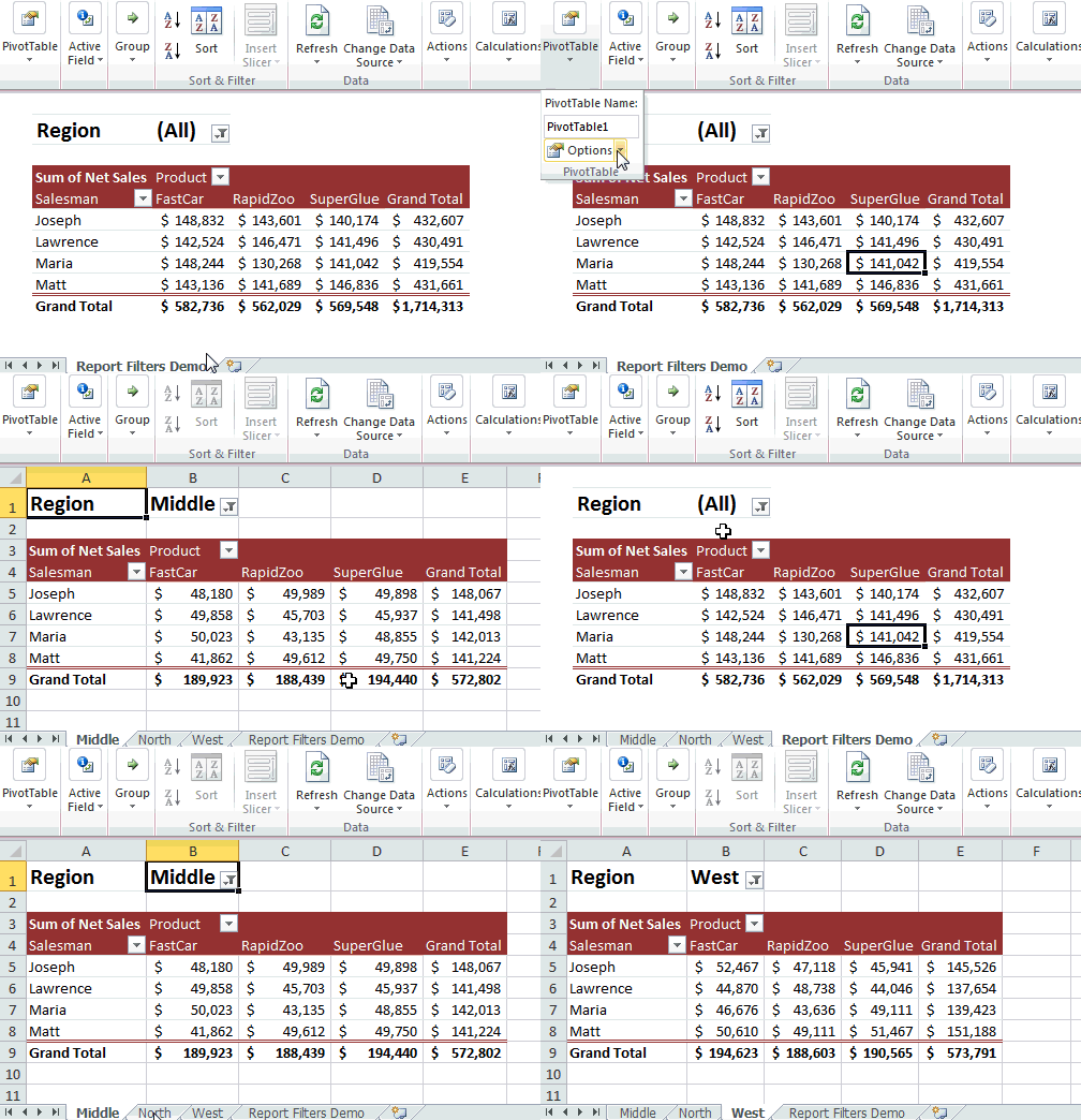
6 - Multiple pages with Report Filters

You got a handy little pivot report that details the performance of a region. Now you want to make similar reports for rest of the 16 regions too.

You can use Report Filters to quickly create all versions of this report in one click. Here is a demo of how report filters work.

Pivot Table Tricks - Video

If you want to view all these tricks + my new haircut, check out below video. 

#evba #etipfree #eama #kingexcel
📤How to Download ebooks: https://www.evba.info/2020/02/instructions-for-downloading-documents.html?m=1