Formula challenge - build answer key for tests

The problem

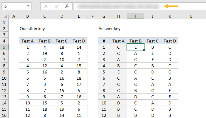
There is one master test (Test A), and three variants (Test B, Test C, and Test D). All 4 tests have the same 19 questions, but arranged in a different order.

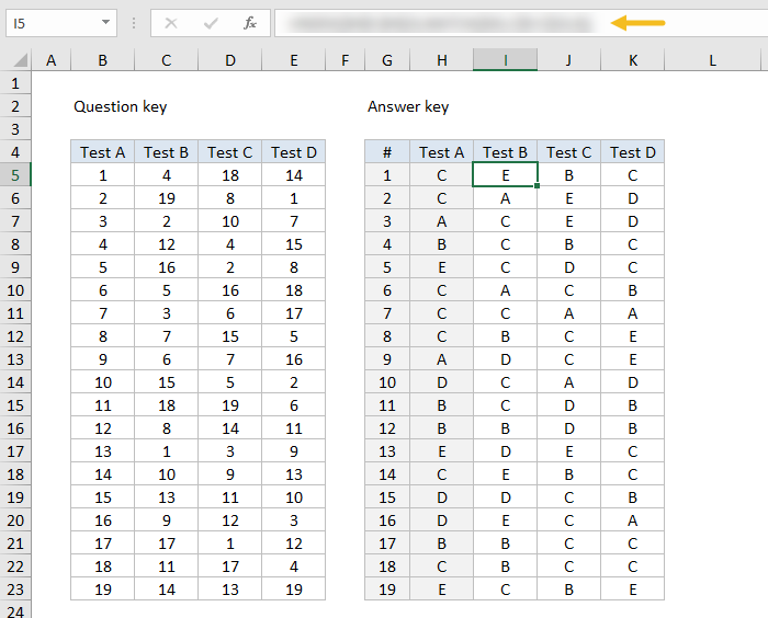
The first table in the screen below is a "question key" and shows how questions in Test A are ordered in the other 3 tests. The second table is an "answer key" that shows the correct answers for all 19 questions in all tests.

Above: Correct answers in I5:K23, formula obscured

For example, the answer to question #1 in Test A is C. This same question appears as question #4 in Test B, so the answer to question #4 in Test B is also C.

The first question in Test B is the same as question #13 in Test A, and the answer to both is E.

The challenge

What formula can be entered in I5 (that's an i as in "igloo") and copied across I5:K23 to find and display the correct answers for Tests B, C, and D?

You'll find the Excel file below. Leave your answer as a comment below.

Hints

1. This problem is challenging to set up. It's very easy to get confused. Remember, the numbers in C5:E23 only tell you where you can find a given question. You still have to find the question after that :)
2. This problem can be solved with INDEX and MATCH, which is explained in this article. Part of the solution involves carefully locking cell references. If you have trouble with these kind of references, practice building the multiplication table shown here. This problem requires carefully constructed cell references!
3. You might find yourself thinking you could do this faster manually. Yes, for a small number of questions. However, with more questions (imagine 100, 500, 1000 questions) the manual approach gets much harder. A good formula will happily handle thousands of questions, and it won't make mistakes :)

Attachments 

 Test answer key challenge.xlsx

HideAnswer (click to expand)

There are two ways to interpret this challenge. When I set up the problem, I was borrowing directly from an example sent to me by a reader. This turns out to be the more challenging approach (Interpretation #2 below), mostly because it's so easy to get confused when trying to understand the table. Below, I explain both interpretations along with formulas that can be used with each.

Interpretation #1 (incorrect)

C5:E23 shows the same questions from test A, simply reordered. So, for example, in Test B...

You can find question #1 from Test A at position #13
You can find question #2 from Test A at position #3
You can find question #3 from Test A at position #7

=INDEX($H$5:$H$23,C5)

With the answers to Test A in the array H5:H23, INDEX simply retrieves a value using the number from column C for row number. Doesn't get much simpler than this. This is not the correct answer for this challenge, but it's a nice example anyway.

Interpretation #2 (correct)

The second interpretation is more complicated. C5:E23 is a key that tells you only where you can find a question from test A. It is not reporting a question number, it is reporting an index of sorts. So, for example, in Test B...

You can find question #1 from Test A at position #4
You can find question #2 from Test A at position #19
You can find question #3 from Test A at position #2

This is a trickier problem. Instead of telling you what question from Test A is in a given position, the key is telling you where you can find the question you seek. The formula below is one correct answer to this problem, since it will return the answers shown in the original challenge.

=INDEX($H$5:$H$23,MATCH($G5,C$5:C$23,0))

Note the mixed references inside MATCH which have been carefully set up to change as needed when the formula is copied across the table.

$G5 - column is locked, row will change
C$5:C$23 - rows are locked, columns will change

#evba #etipfree #eama #kingexcel
📤How to Download ebooks: https://www.evba.info/2020/02/instructions-for-downloading-documents.html?m=1