How to Sort with a Formula in Excel Using SORT and SORTBY Functions
How to Sort with a Formula in Excel Using SORT and SORTBY Functions
Bottom Line: Learn how to use the SORT and SORTBY functions to return a sorted range based on one or more criteria.
Skill Level: Intermediate
Download the Excel File
The file that I work with in the video can be found below. You can also download the “Follow Along” version if you'd like to practice building out the report.
Building an Attendance Dashboard
This post is part 4 of a six-part series explaining how to build an interactive dashboard for attendance. This attendance report was an entry for the Excel Hash competition.
Sort and Rank
In this post we're going to take a look at two more Dynamic Array Functions, SORT and SORTBY. These are great for displaying a list that's ranked in order of performance or chronological order (date, time).
In the case of our example, we are going to sort employees based on the time they spent in the office (duration) for the week. This will rank the employees from those who spent the most time at work to those who spent the least.
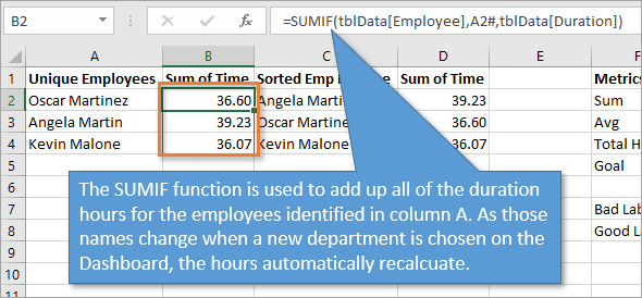
Before we get sorting, however, let me briefly show you how I added all of the duration times together for each employee using the SUMIF function.
The SUMIF Function
SUMIF adds the cells that are specified by a given criteria. It has three arguments. The first is the range of data that the function will search through. In our example, that's the list of employee names.
The second argument is the criteria it's looking for. For this argument, we can specify the spill range we've created that lists only the employees for the department we've identified. In my example, that spill range reference would be A2#.
And finally, the sum range argument is our Duration column. This argument tells Excel to add up all of the duration times for the employees we just identified. So our final formula looks like this:
=SUMIF(tblData[Employee],A2#, tblData[Duration])

The SORTBY Function
Now that we've summed up all of the hours for each employee, we can sort the employees by the number of hours that they worked.
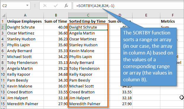
To use the SORTBY function, we just need to identify the data for the three arguments. The first is the Array, which is the set of values that we want to return. In our case it is the unique list of employees, identified by the spill range A2#.
The second argument is By Array, and that is the set of data we want to sort by. We want to sort by the total time each person spent at work, so we use the Sum of Time data, identified by the spill range B2#.
The third and final argument, Sort Order, just specifies how to sort the data. Our choices are ascending or descending. We want to sort in descending order (greatest to smallest), which is represented by -1.
So our SORTBY function would read as follows:
=SORTBY(A2#,B2#,-1)

The SORT Function
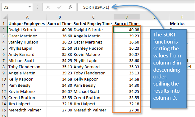
In addition to ranking the employees from most hours of attendance to least, it would also be helpful to list those corresponding hours next to each name. We could accomplish that in many ways, but we will use the SORT function. This is another Dynamic Array Function that returns multiple values in a spill range.
To use SORT, you just need to identify the range that you want to sort, and the order you want to sort it in. (The second argument in the SORT function, sort index, is not needed for our example.)
Our simple formula would look like this:
=SORT (D2#,,-1)

Other Metrics
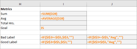
The other formulas on the sheet are fairly basic and are outlined below.
- Sum: =SUM(D2#)
- Avg: =AVERAGE(D2#)
- Good Label: =IF($I$3>=$I$5,$I$3,””)
- Bad Label: =IF($I$3<$I$5,$I$3,””)

Conclusion
In our next video, I will show you how to build out the Attendance Dashboard, now that we have taken care of the calculations and functions behind the scenes.
📤How to Download ebooks: https://www.evba.info/2020/02/instructions-for-downloading-documents.html?m=1


Leave a Comment