How to Create a Dynamic Drop-down List that Automatically Expands

Bottom Line: Learn how to create a drop-down list in a cell using the new UNIQUE function to make the list dynamic.

Skill Level: Intermediate

.

Download the Excel File

The file that I work with in the video can be found below.  You can also download the “Follow Along” version if you'd like to practice building out the report.

 Dunder Mifflin Attendance Report - Follow Along.xlsx (24.4 KB)

 Dunder Mifflin Attendance Report - Final.xlsx (166.6 KB)

Compatibility: This file uses the new Dynamic Array Functions that are only available on the latest version of Office 365. This includes both the desktop and web app versions of Excel.

I have also posted a bonus episode in this series that covers how to make the dashboard with older versions of Excel using pivot tables instead.

Building an Attendance Dashboard

This post is part 5 of a six-part series explaining how to build an interactive dashboard for attendance.  This attendance report was an entry for the Excel Hash competition.  I recommend you check out the first four posts here:

1. How to Use the XOR Function
2. How to Use XLOOKUP for Reverse Order Search
3. Return Multiple Values for a Lookup Formula in Excel with FILTER and UNIQUE
4. How to Sort with a Formula in Excel Using SORT and SORTBY Functions

Data Validation Lists

In this post, we're looking at creating a drop-down list that is dynamic.  In other words, it can expand or contract depending on changes to the source data.  Drop-downs are also called data validation lists, and I've written a post going into more detail about these handy tools that you can check out here: How to Create Drop-Down Lists in Cells.

The drop-down list we're looking at today is part of our attendance dashboard.  It's a list that we can select from in order to filter attendance data by department.

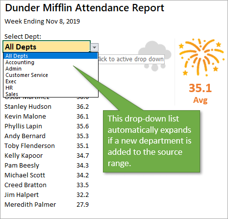
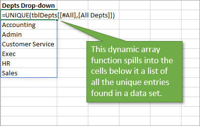
The source of this dynamic data validation list has been created using the UNIQUE function.  UNIQUE is a Dynamic Array Formula that returns all the unique values from a data range.  In other words, it removes duplicates from a data set.

For the list below, this function is scanning the many entries listed in the Department column of our data table and returning only one unique entry for each department.

Setting Up the Data Validation List

To create the data validation list on the Dashboard sheet, start by going to the Data tab on the Ribbon and clicking on the Data Validation icon, which looks like this:

This will bring up the Data Validation window. (If you are working with a merged cell, you may get a pop-up box asking if you want to extend the Data Validation to those other cells. If so, just select Yes.)

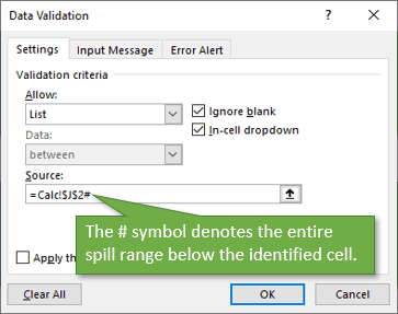
In the Source field, you want to select that list of unique departments that I referred to above. Instead of identifying a range of cells (such as $J$2:$J$8), it's better to reference the spill range ($J$2#). Why? Because then, as departments are added or deleted from the source table, our data validation will automatically update as well.

Phantom Drop-Down Icon

Just a quick side note. One little trick I used in building this dashboard is the inclusion of a drop-down icon that's always visible. Normally this icon only appears when you select the cell that contains the drop-down. But I've found that sometimes it is helpful for users to see that icon no matter where their cursor is on the sheet, so that they know there is a list available that they can select from.

So what I've done is to insert an image of the icon next to the cell in question, and hyperlink it to that cell. That way, when they click on the image, their cursor will move to the cell, and the real drop-down button will appear, covering the ghost icon.

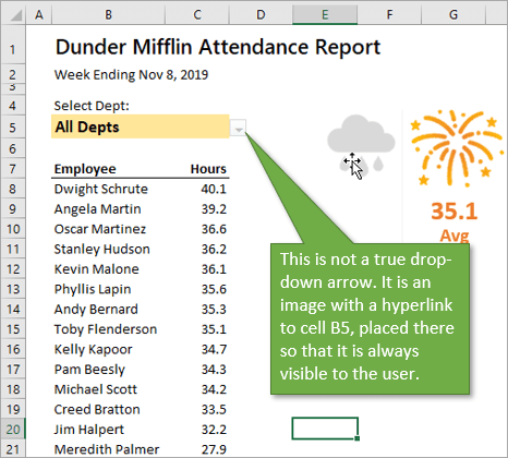
This just makes the worksheet a little more intuitive to someone who hasn't used it before, showing them how they can interact with it.

Here's a blog post explaining how to set that up: Drop-down List Arrow Always Visible for Data Validation.

Populating the Department List

The only thing that remains is to reference the filtered list from the Calc sheet in order for it to show on the Dashboard.

This goes for both the Employee and Hours columns.

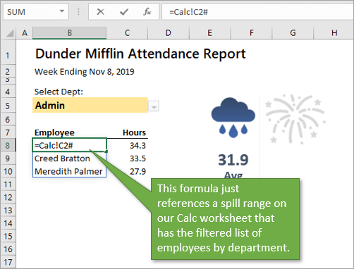
Now, as you select the different departments from the drop-down list, the employees associated with that department will populate in the list.

Related Posts

Here are some other posts I've written that may be of interest to you because they touch on some of the same subjects:

1. For those who do not have Office 365, you can learn how to make dynamic Data Validation Lists without the spill ranges here: How to Add New Rows to Drop-down Lists Automatically.
2. This post will show you how to make secondary drop-down lists that are dependent on the selection made from a primary list. These are called cascading drop-down lists: How to Create Dependent Cascading Drop-down Lists.
3. And finally, this post looks at several other Dynamic Array Formulas like the UNIQUE function that was mentioned above: Dynamic Array Formulas & Spill Ranges.

Conclusion

In our next and final video of the series, e will look at how to create the thundercloud and fireworks icons. These have conditional formatting that causes them to appear grayed out when department hours are above or below a set goal.

#evba #etipfree #eama #kingexcel
📤How to Download ebooks: https://www.evba.info/2020/02/instructions-for-downloading-documents.html?m=1