Excel XLOOKUP Function

Excel XLOOKUP Function

The first powerful function I learnt back in my accounting days was VLOOKUP. It gave me a sense of power and cemented my love of Excel.  Oh, how I wish I’d had the fortune of the new Excel XLOOKUP function back then. XLOOKUP is everything VLOOKUP is and much more.

• XLOOKUP can look up to the left
• XLOOKUP won’t break if columns are inserted or deleted in the lookup array
• XLOOKUP can find the last occurrence of a value
• XLOOKUP defaults to an exact match, so new users won’t accidentally return erroneous data
• XLOOKUP can return a range of cells or a single cell, just like INDEX
• XLOOKUP allows you to specify an alternate value if the lookup value is not found. No more need for IFERROR.

With all this new functionality comes some more arguments, so let’s look at the syntax.

=XLOOKUP( lookup_value, lookup_array, return_array, [if_not_found], [match_mode], [search_mode])

Don’t be put off by the number of arguments in this function because most of the time you’ll only use the first three and it is still way easier than VLOOKUP.

Argument	Description
lookup_value	The value you want to find, or cell containing the item you want to find
lookup_array	The cell range or array you want to search
return_array	The cell range or array containing the value you want returned
[if_not_found]	Optional - the text you want returned in the event a match isn't found. If omitted an error will be returned
[match_mode]	Optional - Defaults to 0 for exact match
[search_mode]	Optional - Defaults to 1 searching first to last
	Options 2 and -2 require the lookup_array to be sorted in ascending or descending order respectively*.

Notes:

*Binary search does not result in faster calculations now that Microsoft have optimised the lookup algorithms.

The lookup_array and return_array must be the same size, otherwise the #VALUE! error will be returned.

If XLOOKUP references another workbook the #REF! error will be returned if the external workbook is closed.

Download Workbook

Download the Excel Workbook and follow along. Note: This is a .xlsx file please ensure your browser doesn't change the file extension on download.

 

Excel XLOOKUP Function Examples

XLOOKUP is a versatile function and will allow the average Excel user to conquer tasks that previously required multiple functions.

1. Simple XLOOKUP

In its most basic form XLOOKUP searches a range of cells and returns an item corresponding to the first match it finds.

The lookup_array doesn’t need to be sorted because XLOOKUP will return an exact match by default.

In English the formula above reads, lookup the value in cell F1, which is Caps, in cells B2:B15 and return the value on the corresponding row in cells C2:C15. If you don’t find an exact match, return an error. This last part is the default behaviour because I didn’t provide a value in the if_not_found argument.

One benefit of this formula over the VLOOKUP equivalent =VLOOKUP(F1,B2:C15,2,0) is that it won’t break if a column is inserted between columns B and C.

2. XLOOKUP does HLOOKUP

Not only does XLOOKUP replace VLOOKUP, but it can also perform HLOOKUPs:

Important: A vertical lookup_array must contain the same number of rows as the return_array and a horizontal lookup_array, as in this example, must contain the same number of columns as the return_array.

3. XLOOKUP does INDEX & MATCH

The formula below crafted by MrExcel himself (aka Bill Jelen), reads: look up Feb in cells A2:A13 and return the value in the range that corresponds with the column Clothing is in.

If you look at the Evaluate Formula dialog box below you can see the second XLOOKUP returns a range:

The fact that XLOOKUP returns a range is what enables us to nest it in the return_array argument.

That said, it’s probably easier to understand an equivalent INDEX & MATCH formula:

=INDEX(B2:D13,MATCH(G2,A2:A13,0),MATCH(F2,B1:D1,0))

Or even the new XMATCH* function which is shorter because it defaults to an exact match meaning the third argument is not required:

=INDEX(B2:D13,XMATCH(G2,A2:A13),XMATCH(F2,B1:D1))

*XMATCH is another new function available to Office 365 users on the Insider channel. For the most part it’s the same as the MATCH function except it defaults to an exact match.

4. XLOOKUP Returns Multiple Columns

In the formula below the return_array argument is columns C and D. With Office 365 XLOOKUP will return multiple values as dynamic arrays allow XLOOKUP to spill the results.

Note: Currently the Excel calc engine can only support spilling XLOOKUP in one direction, either across columns, as in the example above, or down rows as in the example below:

If your XLOOKUP results in two spilled ranges, as in the example below, only the first range will spill:

You can return non-contiguous columns with CHOOSE in the return_array:

Thanks to fellow MVP, Wyn Hopkins for the CHOOSE function idea.

5. XLOOKUP Dynamic Range

Now that we know XLOOKUP can return a range, we can use it to return a dynamic range, which you can name. No more need for OFFSET or INDEX & MATCH to create dynamic named ranges.

In the example below I want to sum the sales values from the start date (G3) to the end date (H3).

Note: My dates are dd/mm/yyyy.

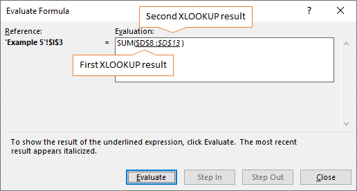
We use two XLOOKUP formulas either side of the colon range operator. The first XLOOKUP returns the first cell in the range and the second XLOOKUP returns the last cell in the range:

=SUM( XLOOKUP(G3,A2:A29,D2:D29) : XLOOKUP(H3,A2:A29,D2:D29) )

You can see how it evaluates in the Evaluate Formula dialog box below:

By now you’re probably thinking that XLOOKUP is a function killer. It has already done away with VLOOKUP, HLOOKUP, INDEX & MATCH and OFFSET, but wait, there’s more! So far, we’ve only used the first 3 arguments. There are still 3 optional arguments to explore.

6. XLOOKUP Error Handling

Back in the early days of VLOOKUP we used IF(ISNA(VLOOKUP… to handle errors. Then came IFERROR which made life simpler and more efficient for Excel. But with XLOOKUP we don’t need any extra functions to handle errors because the fourth argument, if_not_found, allows us to specify a value to be returned in the event XLOOKUP doesn’t find a match.

In the example below I’ve entered the text ‘Not Found’ in the if_not_found argument. Alternatively you can enter numbers, another formula, an array or cell reference.

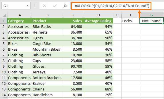
Note: If you omit the if_not_found argument and a match cannot be found, XLOOKUP will return #N/A.

7. XLOOKUP Last Value

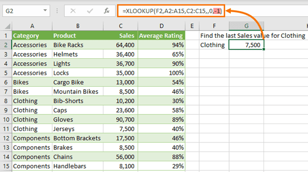
By default, XLOOKUP searches first to last, which is search_mode 1. Using -1 in the search_mode argument tells XLOOKUP to search from the bottom up, thus finding the last matching value. The image below shows XLOOKUP returning the last Sales value for Clothing:

You may have noticed that with 2 or -2 we can also perform binary searches where our lists are sorted:

In earlier versions of Excel, binary searches evaluated more quickly, but according to Microsoft in Office 365 this is no longer the case. As a result, there is no significant benefit to using the binary search options and in fact it’s easier to use 1 or -1 search modes because they don’t require the table to be sorted.

8. XLOOKUP Left

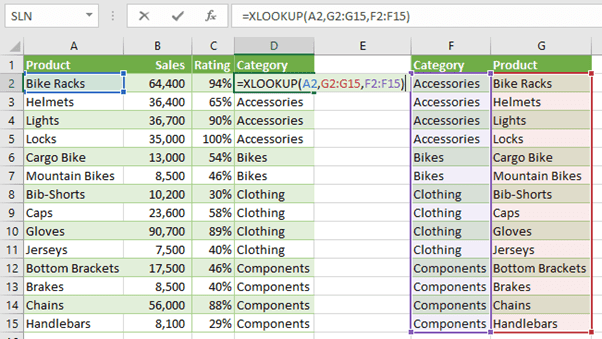
One of the limitations of VLOOKUP is the inability to return values to the left of the lookup column. XLOOKUP isn’t hindered by that limitation, as you can see below:

If you don’t have the XLOOKUP function you can use INDEX & MATCH or the workaround with CHOOSE to trick VLOOKUP into looking up to the left.

9. XLOOKUP Wildcards

VLOOKUP supports wildcards for partial matches by default, which meant looking up words that contained a wildcard like an asterisk e.g. *Alpha, would require the wildcard character to be prefixed by the tilde e.g.:

=VLOOKUP( "~*Alpha", B2:C15, 2, 0)

XLOOKUP only supports wildcards if you specify 2 in the match_mode argument and therefore you don’t need to prefix the wildcard with the tilde:

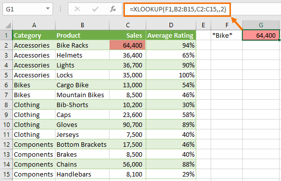
Note: Wildcards cannot be used in binary search mode.

10. XLOOKUP Approximate Match

We can use the match_mode argument to return an approximate match. The formula in the image below uses -1 to find an exact match or the next smallest value in the lookup_range (E2:E7).

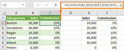
Similarly, specifying 1 in the match_mode argument will return and exact match or the next largest item.

Tip: What’s even better is that the lookup_range doesn’t need to be sorted.
 

Have a great day
#evba #etipfree #eama #kingexcel
📤How to Download ebooks: https://www.evba.info/2020/02/instructions-for-downloading-documents.html?m=1