How to vlookup formula in excel with example
How to vlookup formula in excel with example






 #evba #etipfree #eama #kingexcel
📤How to Download ebooks: https://www.evba.info/2020/02/instructions-for-downloading-documents.html?m=1
Excel VLOOKUP Function

VLOOKUP is an Excel function to lookup and retrieve data from a specific column in table. VLOOKUP supports approximate and exact matching, and wildcards (* ?) for partial matches. The "V" stands for "vertical". Lookup values must appear in the first column of the table, with lookup columns to the right.
Purpose
Lookup a value in a table by matching on the first column
Return value
The matched value from a table.
Syntax
=VLOOKUP (value, table, col_index, [range_lookup])
Arguments
- value - The value to look for in the first column of a table.
- table - The table from which to retrieve a value.
- col_index - The column in the table from which to retrieve a value.
- range_lookup - [optional] TRUE = approximate match (default). FALSE = exact match.
Usage notes
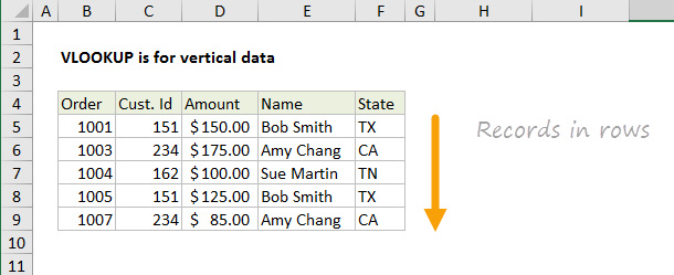
VLOOKUP is designed to retrieve data in a table organized into vertical rows, where each row represents a new record. The "V" in VLOOKUP stands for vertical:

If you have data organized horizontally, use the HLOOKUP function.
VLOOKUP only looks right
VLOOKUP requires a lookup table with lookup values in the left-most column. The data you want to retrieve (result values) can appear in any column to the right:

VLOOKUP retrieves data based on column number
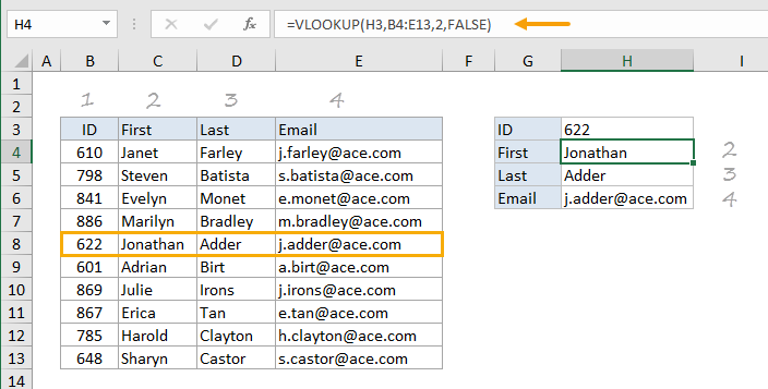
When you use VLOOKUP, imagine that every column in the table is numbered, starting from the left. To get a value from a particular column, provide the appropriate number as the "column index". For example, the column index to retrieve first name below is 2:

=VLOOKUP(H3,B4:E13,2,FALSE) // first
=VLOOKUP(H3,B4:E13,3,FALSE) // last
=VLOOKUP(H3,B4:E13,4,FALSE) // email
VLOOKUP has two matching modes, exact and approximate
VLOOKUP has two modes of matching: exact and approximate, which are controlled by the 4th argument, called "range_lookup". Set range_lookup to FALSE to force exact matching, and TRUE for approximate matching.
Important: range_lookup defaults to TRUE, so VLOOKUP will use approximate matching by default:
=VLOOKUP(value, table, column) // default, approximate match
=VLOOKUP(value, table, column, TRUE) // approximate match
=VLOOKUP(value, table, column, FALSE) // exact match
Example 1: Exact match
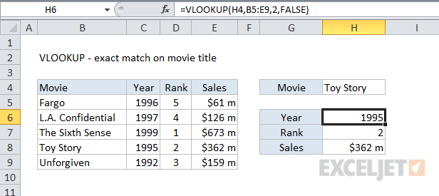
In most cases, you'll probably want to use VLOOKUP in exact match mode. This makes sense when you have a unique key to use as a lookup value, for example, the movie title in this data:

The formula in H6 to find Year based on an exact match of movie title is:
=VLOOKUP(H4,B5:E9,2,FALSE) // FALSE = exact match
Example 2: Approximate match
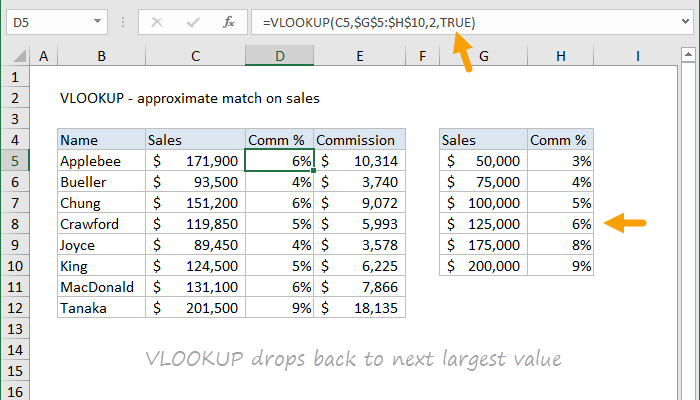
In cases when you want the best match, not necessarily an exact match, you'll want to use approximate mode. For example, below we want to look up a commission rate in the table G5:H10. The lookup values come from column C. In this example, we need to use VLOOKUP in approximate match mode, because in most cases an exact match will never be found. The VLOOKUP formula in D5 is configured to perform an approximate match by setting the last argument to TRUE:

=VLOOKUP(C5,$G$5:$H$10,2,TRUE) // TRUE = approximate match
VLOOKUP will scan values in column G for the lookup value. If an exact match is found, VLOOKUP will use it. If not, VLOOKUP will "step back" and match the previous row.
Note: data must be sorted in ascending order by lookup value when you use approximate match mode with VLOOKUP.
VLOOKUP and #N/A errors
If you use VLOOKUP you will inevitably run into the #N/A error. The #N/A error just means "not found". In practice, there are many reasons why you might see this error. Among the most common:
- The lookup value does not exist in the table
- The lookup value is misspelled, or contains extra space
- Match mode is exact, but should be approximate
- The table range is not entered correctly
- You are copying VLOOKUP, but the table reference is not locked
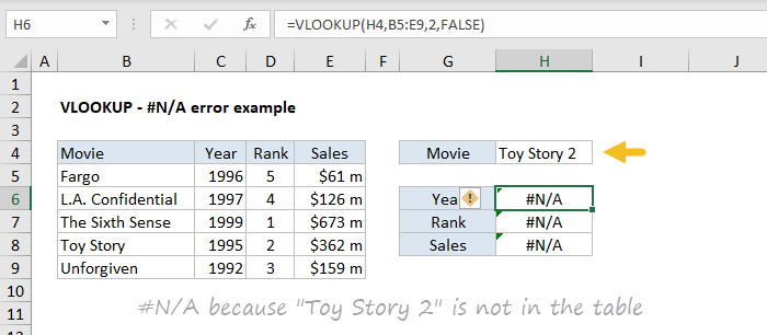
For example, in the example below, the lookup value "Toy Story 2" does not exist in the lookup table, and all three VLOOKUP formulas return #N/A:

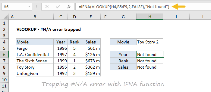
One way to "trap" the NA error is to use the IFNA function:

The formula in H6 is:
=IFNA(VLOOKUP(H4,B5:E9,2,FALSE),"Not found")
The message can be customized as desired. To return nothing (i.e. to display a blank result) when VLOOKUP returns #N/A you can use an empty string like this:
=IFNA(VLOOKUP(H4,B5:E9,2,FALSE),"") // no message
Note: In many cases the #N/A is useful because it tells you something is wrong. Read more here about handling VLOOKUP #N/A errors
More about VLOOKUP
- Detailed VLOOKUP examples
- 23 things you should know about VLOOKUP
- How to find the first or last match
Other notes
- Range_lookup controls whether value needs to match exactly or not. The default is TRUE = allow non-exact match.
- Set range_lookup to FALSE to require an exact match and TRUE to allow a non-exact match.
- If range_lookup is TRUE (the default setting), a non-exact match will cause the VLOOKUP function to match the nearest value in the table that is still less than value.
- When range_lookup is omitted, the VLOOKUP function will allow a non-exact match, but it will use an exact match if one exists.
- If range_lookup is TRUE (the default setting) make sure that lookup values in the first row of the table are sorted in ascending order. Otherwise, VLOOKUP may return an incorrect or unexpected value.
- If range_lookup is FALSE (require exact match), values in the first column of table do not need to be sorted.
VLOOKUP formula examples

VLOOKUP with two client rates
To lookup two different rates for the same client, and calculate a final charge, you can use a formula based on two VLOOKUP functions. In the example shown, the formula in E5 is: =VLOOKUP(B5,rates,2,0)*C5+VLOOKUP(B5,...

Group times into unequal buckets
If you need to group times into buckets, but the buckets are not equal (i.e. 12 AM-7 AM, 7 AM-12 PM, etc.) you can do so with the VLOOKUP function set to approximate match. The problem There are several ways to group...

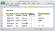
Group arbitrary text values
IF you want to group or classify data based on arbitrary text values, you can use VLOOKUP instead of a long series of nested IF statements. The trick is to build a custom table that will map values to all the groups...

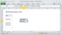
Get first text value in a list
If you need to get the first text value in a list (a one-column range) you can use the VLOOKUP function set to exact match, with a wildcard character for the lookup value. In the example the formula in D7 is: =...

Build hyperlink with VLOOKUP
To create a hyperlink from a lookup, you can use the VLOOKUP function together with the HYPERLINK function. In the example shown, the formula in F5 is: =HYPERLINK(VLOOKUP(E5,link_table,2,0),E5) How this formula...

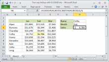
Two-way lookup with VLOOKUP
Preface Inside the VLOOKUP function, the column index argument is normally hard-coded as a static number. However, you can also create a dynamic column index by using the MATCH function to locate the right column....

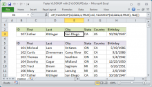
Faster VLOOKUP with 2 VLOOKUPS
With large sets of data, exact match VLOOKUP can be painfully slow, but you can make VLOOKUP lightening fast by using two VLOOKUPS, as explained below. Notes: If you have a smaller set of data, this approach is...

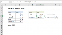
How to fix the #N/A error
About the #N/A error The #N/A error appears when something can't be found or identified. It is often a useful error, because it tells you something important is missing – a product not yet available, an employee name...

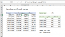
Commission split formula example
To calculate a commission, and split the Commission between Agent and Broker according to a pre-established schedule, you can use the VLOOKUP function. In the example shown, the formula in D5 is: =C5*VLOOKUP(B5,...

VLOOKUP with multiple critiera
The VLOOKUP function does not handle multiple criteria natively. However, if you have control over source data, you can use a helper column to join multiple fields together, and use these fields like multiple criteria...

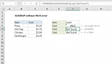
VLOOKUP without #N/A error
To hide the #N/A error that VLOOKUP throws when it can't find a value, you can use the IFERROR function to catch the error and return any value you like. How the formula works When VLOOKUP can't find a value in a...

Dynamic lookup table with INDIRECT
To allow a dynamic lookup table, you can use the INDIRECT function with named ranges inside of VLOOKUP. In the example shown the formula in G5 is: =VLOOKUP(F5,INDIRECT(E5),2,0) Background The purpose of this formula...

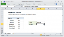
Map text to numbers
To map or translate text inputs to arbitrary numeric values, you can use the VLOOKUP function with a simple table. In the example, we need to map five text values (statuses) to numeric status codes as follows...

Multiple chained VLOOKUPs
If you need to perform multiple lookups sequentially, based on whether the earlier lookups succeed or not, you can chain one or more VLOOKUPs together with IFERROR. In the example shown, the formula in L5 is: =...

Win loss points calculation
To assign points based on win/loss/tie results for a team, you can use a simple VLOOKUP formula, or a nested IF formula, as explained below. In the example shown, the formula in D5 is: =VLOOKUP(C5,points_table,2,0)...
📤How to Download ebooks: https://www.evba.info/2020/02/instructions-for-downloading-documents.html?m=1


Leave a Comment