Excel 2020: Create Interactive Charts

It is easy to create interactive charts without using VBA. By default, if you hide rows in Excel, those rows will be hidden in the chart. The technique is to build a chart with every possible customer and then use a slicer or a filter to hide all except one of the customers.

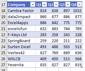
Say that you have the following list of customers. Make the data into a table by using Ctrl+T.

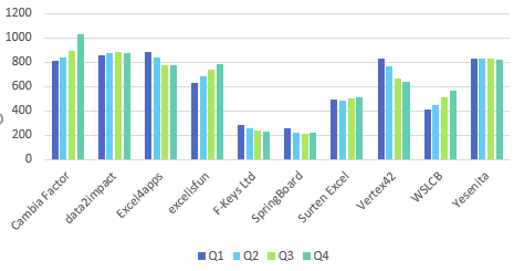
Select the table and insert a chart. In most cases, Excel will create the wrong chart, with customers along the X-axis.

---

Click the Switch Row/Column icon in the Chart Tools Design tab of the Ribbon.

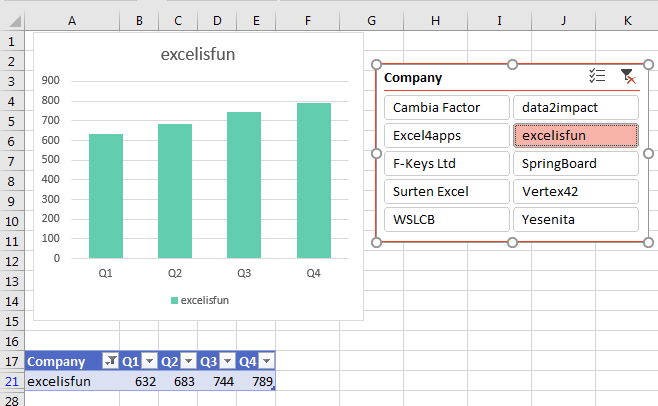
Select one cell in the table. In Excel 2013 or newer, go to the Insert tab of the Ribbon and choose Slicer. In Excel 2010 or earlier, you have to use the Company dropdown in A17 to choose a single company.

By default, every slicer starts as a single column in the middle of the screen. Plan on dragging the slicer to a new location and size. While the slicer is selected, you can use the Columns spin button near the right side of the Slicer Tools Options tab of the Ribbon to change the number of columns in the slicer.

In the following figure, choose one customer from the slicer and the chart updates to show just that one customer.

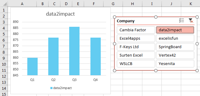
Choose a different customer, and the chart updates for that customer.

#evba #etipfree #eama #kingexcel
📤How to Download ebooks: https://www.evba.info/2020/02/instructions-for-downloading-documents.html?m=1