What is an INDIRECT Function in Excel?

January 20, 2020 Excel tips,

What is an INDIRECT Function in Excel?

The INDIRECT Function in Excel helps you to return a reference to a range. Even when you insert Rows or Columns in a Worksheet the reference you created won’t change. This will help you to create a reference from letters and numbers in other cells.

How INDIRECT Function in Excel Works with an Example

The INDIRECT function is useful when you want to return a value, based on a text string. Example: You’ll be able to see the list of food items and their Consumption by Countries such as USA, China and Japan. The quantity is in Million i.e. 1 Million=10,00,000

Problem: You need to find out:

An independent Cell Value
SUM consumption of the Food items of USA
MAX Value of Food Consumption of Japan
MIN Value of Food Consumption of CHINA

Question: How will you find the Values?

Solution: INDIRECT Formula will help you get this in minutes

INDIRECT Formula to find an independent Cell Value

In the Cell F3, Type =INDIRECT(for ref_text give the reference of the above Cell, Select F2) i.e. =INDIRECT(F2)
You get #REF! (This is because there was no Cell Value assigned to the Cell F2)
Select C5 and Enter C5 as the Cell Value at the place of F2. You get Value 150

(The Error text disappears and you get the Value 150 i.e. the Value of Silk Consumption in China)

INDIRECT Formula to find a Sum consumption

Select the range of Cells for the Columns USA, CHINA and JAPAN
Provide a Table Name to USA, CHINA and JAPAN respectively in the NAME BOX
Type the name USA in the Cell F2
In the Cell F3, Type =SUM(INDIRECT(F2))

Note 1: Don’t forget to close the Bracket for SUM & INDIRECT both

Note 2: If you don’t Select the Table Range and Name your Table then Typing USA won’t give the SUM in Excel. You must Give your Table a name in the NAME BOX

Press Enter. You’ll get the Value 1250

(You can Cross-Check the Total by Calculating the Total Values of USA. The Answer remains same)

Note: You can change the Country Name to China and Japan Respectively to get the Sum of the Country

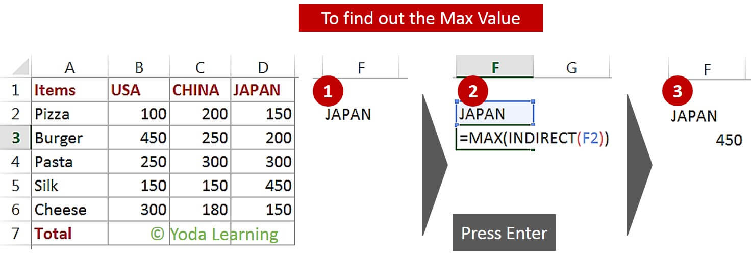
INDIRECT Formula to find MAX Value

In the Cell F2, Type JAPAN
In the Cell F3, Type =MAX(=INDIRECT(F2))
Press Enter. You’ll get the Value 450

Note: If you don’t Select the Table Range and Name your Table then Typing USA won’t give the SUM in Excel. You must give your Table a name in the NAME BOX

(You can Cross Check the MAX Value by Checking out the Column of Japan. The Answer remains same)

INDIRECT Formula to find MIN Value

In the Cell F2, Type CHINA
In the Cell F3, Type =MIN(=INDIRECT(F2))
Press Enter. You’ll get the Value 150

Note: If you don’t Select the Table Range and Name your Table then Typing USA won’t give the SUM in Excel. You must give your Table a name in the NAME BOX

(You can Cross-Check the MIN Value by Checking out the Column of Japan. The Answer remains same)

Wish to learn about:

‘Excel reference cell in another sheet dynamically’?

Excel INDIRECT function – syntax and basic uses

As you understand from the Word, ‘Excel INDIRECT’, it helps to indirectly reference cells, ranges, other sheets or workbooks.

In other words, The INDIRECT function in Excel makes it easy for you to create an Excel dynamic cell reference or range reference. You do not have to do the “hard-coding” of the references into your Excel formulas.

This results in the change of a Cell Reference within a formula without changing the formula itself. More importantly, these indirect references in the INDIRECT Formula in Excel do not change when a new row or column is added or inserted in the worksheet. Also, the Cell Reference remains the same when you delete the existing Rows and Columns. When some formulas get extended you can use wrap text in Excel

If you wish to Write an INDIRECT Function in Excel, you need to understand the Basics of Function Arguments.

Download Sample File

What if your Indirect formula not working?

Situation: You’re using the indirect formula in Excel to pull data of other tabs.

These tab names are compiled and placed on a tab through VBA code (this is a clear cut and paste)

Problem: The Indirect formula is unable to calculate because what I am assuming is the format of the data which is present in column B

It is observed that: Whenever you type over the data (which is exactly the same) this excel formula works.

Solution: Before you overwrite, you need to check:

If there are unseen Whitespace Characters in the Cell
If something is Misspelled

If this doesn’t work then, you can try this:

=IF(ISERROR(INDIRECT(TRIM($B2)&”!U2″)),””,INDIRECT(TRIM($B2)&”!U2″))

#evba #etipfree #kingexcel
📤You download App EVBA.info installed directly on the latest phone here : https://www.evba.info/p/app-evbainfo-setting-for-your-phone.html?m=1