Using Conditional Formatting to highlight range of percentages in Excel

With conditional formatting feature, Excel makes even the numeric bits easy to understand with visual aids. Conditional formatting lets you format the cell and text within in relation to particular condition.

Suppose you want your data to appear like this:

• Less than 0% = Red
• Greater than 0% but equal to 5% = Yellow
• Greater than 5% = Green

You can get it done easily even without a formula by defining three specific rules using conditional formatting dialogue box. Following steps will help you get it done easily:

Step 1: Have your data prepared and percentages calculated. Usually we don’t have negative percentages but to represent the decrease or adverse variance we use it. This helps us not only show that the figure is negative but also the extent of it.

For illustration purposes I have a very simple data. In column A I have a budgeted data and in column B I have actual data.

Step 2: In column C put this formula in cell C2:

=(B2/A2)-1

Press Enter and drag the fill handle down to row 6. All numbers will be in decimals.

Step 3: Select the range from C2 to cell C6 and hit Ctrl+Shift+5 to apply the percentage formatting. Once done the numbers will appear in percentages.

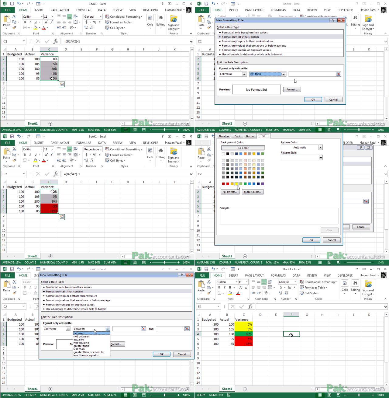
Step 4: Having C2:C6 range still selected go to Home tab > Styles group > click conditional formatting drop down button > hit New rule

Step 5: Click New rule button. Select the option “Format only cells that contain”. Change the second drop down under “Format only cells with” to less than and type in 0%. Click format button > fill tab and select red color. Press OK to close the dialogue box.

Step 6: Click the new rule button again. Select the option “Format only cells that contain”. Change the second drop down under “Format only cells with” to between and type in 0% in the first field and 5% in the second field. Click the format button and select a yellow color under the fill tab. Press OK to close the dialogue box

Step 7: Click the new rule button again. Select the option “Format only cells that contain”. Change the second drop down under “Format only cells with” to Greater than and type in 5% in the field. Click the format button and select green color under the fill tab. Click OK to close the dialogue box.

Step 8: Click Apply button and TADA!!!

Following animation will walk you through the whole process:

You have your percentages color coded to easily know what type of variance you are assessing without stressing your mathematics skills 

#evba #etipfree #kingexcel
📤You download App EVBA.info installed directly on the latest phone here : https://www.evba.info/p/app-evbainfo-setting-for-your-phone.html?m=1