Separate First and Last Name in Excel (Split Names Using Formulas)

Split Names Using Text to Columns

Text to Columns functionality in Excel allows you to quickly split text values into separate cells in a row.

For example, suppose you have the dataset as shown below and you want to separate the first and last name and get these in separate cells.

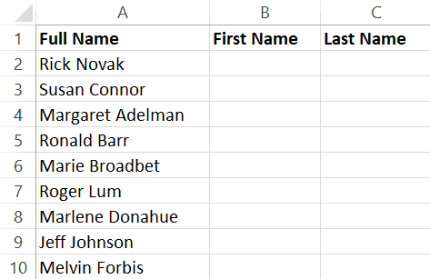
Below are the steps to separate the first and last name using Text to Columns:

1. Select all the names in the column (A2:A10 in this example)
2. Click the ‘Data’ tab
3. In the ‘Data Tools’ group, click on the ‘Text to Columns’ option.
4. Make the following changes in the Convert Text to Column Wizard:
   1. Step 1 of 3: Select Delimited (this allows you to use space as the separator) and click on Next
   2. Step 2 of 3: Select the Space option and click on Next
   3. Step 3 of 3: Set B2 as the destination cell (else it will overwrite the existing data)
5. Click on Finish

The above steps would instantly split the names into first and last name (with first names in column B and last name in column C).

Note: In case there is any data in the cells already (the ones where Text to Columns output is expected), Excel will show you a warning letting you know that there is some data already in the cells. You can choose to overwrite the data or cancel Text to Columns and manually remove it first.

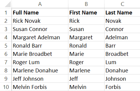
Once done, you can delete the full name data if you want.

A few things to know when using Text to Columns to separate first and last names in Excel:

1. The result of this is static. This means that in case you have new data or the original data has some changes, you need to do this all over again to split the names.
2. If you only want the First name or only the Last name, you can skip the columns you don’t want in step 3 of the ‘Text to Column Wizard’ dialog box. To do this, select the column in the preview that you want to skip and then select the ‘Do not import column (skip)’ option.
3. In case you don’t specify the destination cell, Text to Column will overwrite the current column

Text to Columns option is best suited when you have consistent data (for example all names have first and last name only or all names have a first, middle, and last names).

In this example, I have shown you how to separate names that have space as the delimiter. In case the delimiter is a comma or a combination of comma and space, you can still use the same steps. In this case, you can specify the delimiter in Step 2 of 3 of the wizard. There is already an option to use the comma as the delimiter, or you can select ‘Other’ option and specify a custom delimiter as well.

While Text to Columns is a fast and efficient way to split names, it’s suited only when you want the output to be a static result. In case you have a dataset that may expand or change, you are better off using formulas to separate the names.

Separate First, Middle, and Last Names Using Formulas

Formulas allow you to slice and dice the text data and extract what you want.

In this section, I will share various formulas you can use to separate name data (based on how your data is structured).

Below are the three formulas you can use to separate first, middle, and last name (explained in detail later in the following sections).

Formula to get the first name:

=LEFT(A2,SEARCH(" ",A2)-1)

Formula to get the middle name:

=MID(A2,SEARCH(" ",A2)+1,SEARCH(" ",SUBSTITUTE(A2," ","@",1))-SEARCH(" ",A2))

Formula to get the last name:

=RIGHT(A15,LEN(A15)-SEARCH("@",SUBSTITUTE(A15," ","@",LEN(A15)-LEN(SUBSTITUTE(A15," ","")))))

Get the First Name

Suppose you have the dataset as shown below and you want to quickly separate the first name in one cell and last name in one cell.

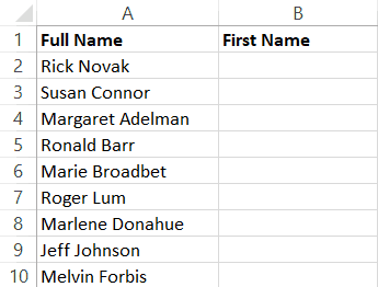
The below formula will give you the first name:

=LEFT(A2,SEARCH(" ",A2)-1)

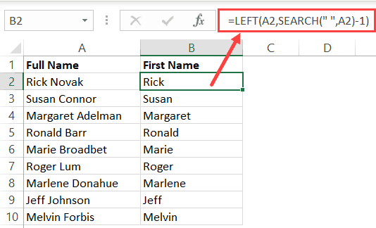
The above formula uses the SEARCH function to get the position of the space character in between the first and last name. The LEFT function then uses this space position number to extract all the text before it.

This is a fairly straight forward use of extracting a part of the text value. Since all we need to do is identify the first space character position, it doesn’t matter whether the name has any middle name or not. The above formula is going to work just fine.

Now, let’s get a little more advanced with each example.

Get the Last Name

Let’s say you have the same dataset and this time you need to get the last name.

The below formula will extract the last name from the above dataset:

=RIGHT(A2,LEN(A2)-SEARCH(" ",A2))

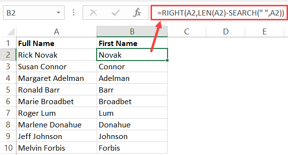
Again, quite straightforward.

This time, we first find the space character position, which is then used to find out the number of characters that are left after space (which would be the last name).

This is achieved by subtracting the position value of the space character with the total number of characters in the name.

This number is then used in the RIGHT function to fetch all these characters from the right of the name.

While this formula works great when there is only the first and last name, it wouldn’t work in case you also have a middle name. This is because we only accounted for one space character (between first and last name). Having a middle name adds more space characters to the name.

To fetch the last name when you have a middle name as well, use the below formula:

=RIGHT(A15,LEN(A15)-SEARCH("@",SUBSTITUTE(A15," ","@",LEN(A15)-LEN(SUBSTITUTE(A15," ","")))))

Now, this has started to become a bit complex… isn’t it?

Let me explain how this works.

The above formula first finds the total number of space characters in the name. This is done by getting the length of the name with and without the space character and then subtracting the one without space from the one with space. This gives the total number of space characters.

The SUBSTITUTE function is then used to replace the last space character with an ‘@’ symbol (you can use any symbol – something which is unlikely to occur as a part of the name).

Once the @ symbol has been substituted in place of the last space character, you can easily find the position of this @ symbol. This is done using the SEARCH function.

Now all you need to do is extract all the characters to the right of this @ symbol. This is done by using the RIGHT function.

Get the Middle Name

Suppose you have the dataset as shown below and you want to extract the middle name.

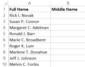
The following formula will do this:

=MID(A2,SEARCH(" ",A2)+1,SEARCH(" ",SUBSTITUTE(A2," ","@",1))-SEARCH(" ",A2))

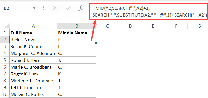
The above formula uses the MID function, which allows you to specify a start position and the number of characters to extract from that position.

The start position is easy to find using the SEARCH function.

The hard part is to find how many characters to extract after this start position. To get this, you need to identify how many characters are there from the start position to the last space character.

This can be done by using the SUBSTITUTE function and replace the last space character with an ‘@’ symbol. Once this is done, you can easily use the SEARCH function to find the position of this last space character.

Now that you have the starting position and the position of the last space, you can easily fetch the middle name by using the MID function.

One of the benefits of using a formula to separate the names is that the result is dynamic. So in case, your dataset expands and more names are added to it or if some names change in the original dataset, you don’t need to worry about the resulting data.

Separate Names Using Find and Replace

I love the flexibility that comes with ‘Find and Replace‘ – because you can use wild card characters in it.

Let me first explain what’s a wild card character.

A wildcard character is something that you can use instead of any text. For example, you can use an asterisk symbol (*) and it will represent any number of characters in Excel. To give you an example, if I want to find all the names that start with the alphabet A, I can use A* in find and replace. This will find and select all the cells where the name starts with A.

If you’re still not clear, don’t worry. Keep reading and the next few examples will make it clear what wildcard characters are and how to use these to quickly separate names (or any text values in Excel).

In all the examples covered below, make sure you create a backup copy of the dataset. Find and Replace changes the data on which it’s used. It’s best to copy and paste the data first and then use Find and Replace on the copied dataset.

Get the First Name

Suppose you have a dataset as shown below and you want to get the first name only.

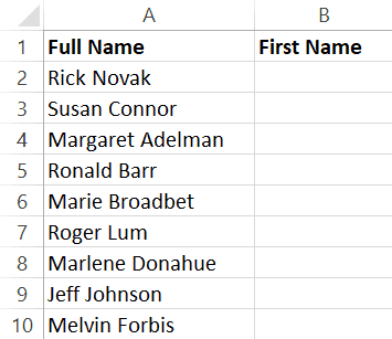
Below are the steps to do this:

1. Copy the name data in Column A and paste it in Column B.
2. With the data in Column B selected, click the Home tab
3. In the Editing group, click on Find & Select.
4. Click on Replace. This will open the ‘Find and Replace’ dialog box.
5. In the ‘Find and Replace’ dialog box, enter the following
   1. Find what:  * (space character followed by the asterisk symbol)
   2. Replace with: leave this blank
6. Click on Replace All.

The above steps would give you the first name and remove everything after the first name.

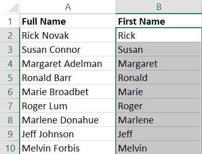
This works even if you have names that have a middle name.

Pro Tip: The keyboard shortcut to open the Find and Replace dialog box is Control + H (hold the control key and then press the H key).

Get the Last Name

Suppose you have a dataset as shown below and you want to get the last name only.

Below are the steps to do this:

1. Copy the name data in Column A and paste it in Column B.
2. With the data in Column B selected, click the Home tab
3. In the Editing group, click on Find & Select.
4. Click on Replace. This will open the ‘Find and Replace’ dialog box.
5. In the ‘Find and Replace’ dialog box, enter the following
   1. Find what: *  (asterisk symbol followed by a space character)
   2. Replace with: leave this blank
6. Click on Replace All.

The above steps would give you the last name and remove everything before the first name.

This works even if you have names that have a middle name.

Remove the Middle Name

In case you only want to get rid of the middle name and only have the first and the last name, you can do that using Find and Replace.

Suppose you have a dataset as shown below and you want to remove the middle name from these.

Below are the steps to do this:

1. Copy the name data in Column A and paste it in Column B.
2. With the data in Column B selected, click the Home tab
3. In the Editing group, click on Find & Select.
4. Click on Replace. This will open the ‘Find and Replace’ dialog box.
5. In the ‘Find and Replace’ dialog box, enter the following
   1. Find what: * (space character followed by the asterisk symbol followed by the space character)
   2. Replace with:  (just put a space character here)
6. Click on Replace All.

The above steps would remove the middle name from a full name. In case some names don’t have any middle name, they would not be changed.

Separate Names Using Flash Fill

Flash fill was introduced in Excel 2013 and makes it really easy to modify or clean a text data set.

And when it comes to separating names data, it’s right up in Flash Fill’s alley.

The most important thing to know when using Flash Fill is that there needs to a pattern that flash fill can identify. Once it has identified the pattern, it will easily help you split names in Excel (you will get more clarity on this when you go through a few examples below).

Get the First or the Last Name from Full Name

Suppose you have a dataset as shown below and you want to get only the first name.

1. In the adjacent cell, manually type the first name from the full name. In this example, I would type Rick.
2. In the second cell, manually type the first name from the adjacent cell’s name. While you’re typing, you will see Flash Fill show you a list of the first name automatically (in gray).
3. When you see the names in grey, quickly glance through it to make sure it’s showing the right names. If these are right, hit the enter key and Flash Fill will automatically fill the rest of the cells with the first name.

Flash Fill needs you to give it a pattern that it can follow when giving you the modified data. In our example, when you type the first name in the first cell, Flash Fill can’t figure out the pattern.

But as soon as you start entering the First name in the second cell, Flash Fill understands the pattern and shows you some a suggestion. If the suggestion is correct, just hit the enter key.

And if it’s not correct, you can try entering manually in a few more cells and check if Flash Fill is able to discern the pattern or not.

Sometimes, you may not see the pattern in gray (as shown in step 2 above). If that’s the case, follow the below steps to get the Flash Fill result:

1. Enter the text manually in two cells.
2. Select both these cells
3. Hover the cursor on the bottom-right part of the selection. You will notice that the cursor changes to a plus icon
4. Double click on it (mouse left-key). This will fill all the cells. At this point in time, the results are likely incorrect and not what you expected.
5. At the bottom right of the resulting data, you will see a small Auto-Fill icon. Click on this Auto-fill icon
6. Click on Flash Fill

The above steps would give you the result from Flash Fill (based on the pattern it has deduced).

You can also use Flash Fill to get the last name or the middle name. In the first two cells, enter the last name (or the middle name) and flash fill will be able to understand the pattern

Rearrange Name Using Flash Fill

Flash Fill is a smart tool and it can decipher slightly complex pattern as well

For example, suppose you have a dataset as shown below and you want to rearrange the name from Rick Novak to Novak, Rick (where the last name comes first followed by a comma and then the first name).

Below are the steps to do this:

1. In the adjacent cell, manually type Novak, Rick
2. In the second cell, manually type Connor, Susan. While you’re typing, you will see Flash Fill show you a list of the names in the same format (in gray).
3. When you see the names in grey, quickly glance through it to make sure it’s showing the right names. If these are right, hit the enter key and Flash Fill will automatically fill the rest of the cells with the names in the same format.

Remove the Middle Name (or Just get the middle name)

You can also use Flash Fill to get rid of the middle name or get only the middle name.

For example, suppose you have a dataset as shown below and you want to get only the first and the last name and not the middle name.

Below are the steps to do this:

1. In the adjacent cell, manually type Rick Novak
2. In the second cell, manually type Susan Connor. While you’re typing, you will see Flash Fill show you a list of the names in the same format (in gray).
3. When you see the names in grey, quickly glance through it to make sure it’s showing the right names. If these are right, hit the enter key and Flash Fill will automatically fill the rest of the cells with the names without the middle name.

Similarly, if you only want to get the middle names, type the middle name in the first two cells and use Flash Fill to get the middle name from all the remaining names.

The examples shown in this tutorial uses names while manipulating the text data. You can use the same concepts to also work with other formats of data (such as addresses, product names, etc.)

#evba #etipfree #kingexcel
📤You download App EVBA.info installed directly on the latest phone here : https://www.evba.info/p/app-evbainfo-setting-for-your-phone.html?m=1