Perform VLOOKUP with 2 lookup values

Perform VLOOKUP with 2 lookup values

by MF

4 different ways to perform LOOKUP with 2 lookup values

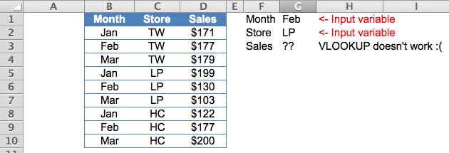
We know that VLOOKUP is very useful. At the same time, we know that VLOOKUP has its limitations. E.g. VLOOKUP only looks from left to right; VLOOKUP only handle one lookup value.  For a simple situation shown below, VLOOKUP doesn’t seem to work (directly).

No worry. There are at least four workarounds!

1. Using a helper column
2. Using CHOOSE to recreate the Table Array for VLOOKUP
3. Using INDEX, MATCH and = Operator
4. Using SUMPRODUCT

Let’s start with the basic.

1. Using a helper column

Most of the time, complicated problem will become easier and manageable when it is broken down into small pieces. Same applies in formula building in Excel.
Take below example:

By CONCATENATING “Month” and “Store” in column A (note: better to put the helper column to the left of the original Table as VLOOKUP looks from left to right.), we create the lookup value required in column A.  As a result, with the helper column A (which could be hidden later), the problem can be solved easily by

=VLOOKUP(G1&G2,$A$2:$D$10,4,FALSE)

Note: we need to combine the Month (G1) and Store (G2) as the lookup value

Non-helper column approach

Well, for any reason a helper column is not an option, we may do it by array formula. At least two different ways to perform the job:

2) Using CHOOSE to recreate the Table Array for VLOOKUP

This is a bit advance. The tricky part is to re-create the Table Array that is suitable for VLOOKUP by using CHOOSE.
CHOOSE({1,2},B2:B10&C2:C10,D2:D10) does two things

1. Combine “Month” and “Store” into a single array as “JanTW”;”FebTW”, etc……
2. Join the two arrays into a “table” of two columns

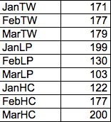
When we evaluate the result of the above CHOOSE (by selecting the whole CHOOSE formula in the formula bar and then press F9, we get the following result:

{"JanTW",171;"FebTW",177;"MarTW",179;"JanLP",199;"FebLP",130;"MarLP",103;"JanHC",122;"FebHC",177;"MarHC",200}

To visualize it in a Table format, it looks like the below:

Now the whole formula makes sense:

=VLOOKUP(G1&G2,CHOOSE({1,2},B2:B10&C2:C10,D2:D10),2,FALSE)
 CTRL SHIFT ENTER (not just ENTER)

IMPORTANT: As this is an array formula, we have to input CTRL SHIFT ENTER to tell Excel that we are going to input array formula. You will see the {} in the formula bar if array formula is input successfully.

• • Note: For both 1) and 2), the robust way to combine the lookup values should include a delimiter in between, e.g. A1 & “|” & B1 . 

3) Using INDEX, MATCH and = Operator

=INDEX(D2:D10,MATCH(1,(B2:B10=G1)*(C2:C10=G2),0))
 CTRL SHIFT ENTER

This formula actually looks more intuitive. How?

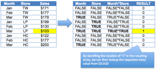
First let’s understand what the (B2:B10=G1)*(C2:C10=G2) does?

• B2:B10=G1 asks Excel to evaluate if B2=G1, if yes, it returns TRUE; if no, it returns FALSE. Then do the same for B3=G1, B4=G1…… until B10=G1. An array of TRUE/FALSE will be the result.
• C2:C10=G2 basically does the same thing but look at different values.

When we compare the two array of TRUE/FALSE by multiplying them, only TRUE * TRUE gives the result of 1 (TRUE).  A picture tells more. Let’s take a look at the screenshot below:

Bingo, we can identify the row that meets both lookup values.

Now you should be able to use MATCH to identify the position of the matching values. Then use INDEX to return the result required.

• =INDEX(D2:D10,MATCH(1,(B2:B10=G1)*(C2:C10=G2),0)) gives
• =INDEX(D2:D10,MATCH(1,{0;0;0;0;0;1;0;0;0},0) gives
• =INDEX(D2:D10,6) returns
• $103, the correct result!

4) Using SUMPRODUCT

SUMPRODUCT is a powerful function in Excel. I am going to write separate posts about SUMPRODUCT later. Although SUMPRODUCT seems to work in our example, it actually fails if the result we want is text instead of value.

To understand that, we have to understand how SUMPRODUCT behaves. If you want to know more about SUMPRODUCT, stay tuned!

So, which one do I use?

Although options 2) and 3) works fine, I prefer option 1) under normal circumstance.  Why?

In daily work life, I believe it is more important to build a spreadsheet that is manageable and readable by most users (including myself)… Not every one in workplace is Excel guru. If every one is, we don’t have to spend so much time to fight with spreadsheets.

As such, let’s obey the KISS principle whenever possible.

#evba #etipfree #kingexcel
📤You download App EVBA.info installed directly on the latest phone here : https://www.evba.info/p/app-evbainfo-setting-for-your-phone.html?m=1