Highlight Rows Based on a Cell Value in Excel (Conditional Formatting)

In case you prefer reading written instruction instead, below is the tutorial.

Conditional Formatting allows you to format a cell (or a range of cells) based on the value in it.

But sometimes, instead of just getting the cell highlighted, you may want to highlight the entire row (or column) based on the value in one cell.

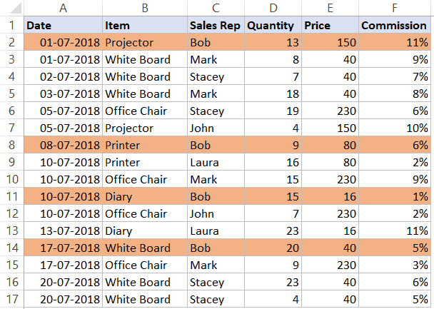
To give you an example, below I have a dataset where I have highlighted all the rows where the name of the Sales Rep is Bob.

In this tutorial, I will show you how to highlight rows based on a cell value using conditional formatting using different criteria.

Click here to download the Example file and follow along.

This Tutorial Covers:

• Highlight Rows Based on a Text Criteria
• Highlight Rows Based on a Number Criteria
• Highlight Rows Based on a Multiple Criteria (AND/OR)
• Highlight Rows in Different Color Based on Multiple Conditions
• Highlight Rows Where Any Cell is Blank
• Highlight Rows Based on Drop Down Selection

Highlight Rows Based on a Text Criteria

Suppose you have a dataset as shown below and you want to highlight all the records where the Sales Rep name is Bob.

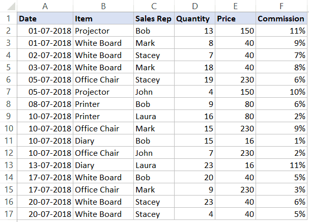
Here are the steps to do this:

1. Select the entire dataset (A2:F17 in this example).
2. Click the Home tab.
3. In the Styles group, click on Conditional Formatting.
4. Click on ‘New Rules’.
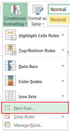
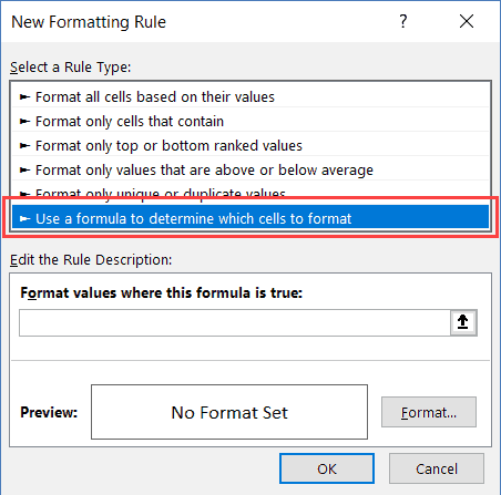
5. In the ‘New Formatting Rule’ dialog box, click on ‘Use a formula to determine which cells to format’.
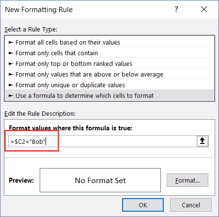
6. In the formula field, enter the following formula: =$C2=”Bob”
7. Click the ‘Format’ button.
8. In the dialog box that opens, set the color in which you want the row to get highlighted.
9. Click OK.

This will highlight all the rows where the name of the Sales Rep is ‘Bob’.

Click here to download the Example file and follow along.

How does it Work?

Conditional Formatting checks each cell for the condition we have specified, which is =$C2=”Bob”

So when it’s analyzing each cell in row A2, it will check whether the cell C2 has the name Bob or not. If it does, that cell gets highlighted, else it doesn’t.

Note that the trick here is to use a dollar sign ($) before the column alphabet ($C1). By doing this, we have locked the column to always be C. So even when cell A2 is being checked for the formula, it will check C2, and when A3 is checked for the condition, it will check C3.

This allows us to highlight the entire row by conditional formatting.

Related: Absolute, Relative, and Mixed references in Excel.

Highlight Rows Based on a Number Criteria

In the above example, we saw how to check for a name and highlight the entire row.

We can use the same method to also check for numeric values and highlight rows based on a condition.

Suppose I have the same data (as shown below), and I want to highlight all the rows where the quantity is more than 15.

Here are the steps to do this:

1. Select the entire dataset (A2:F17 in this example).
2. Click the Home tab.
3. In the Styles group, click on Conditional Formatting.
4. Click on ‘New Rules’.
5. In the ‘New Formatting Rule’ dialog box, click on ‘Use a formula to determine which cells to format’.
6. In the formula field, enter the following formula: =$D2>=15
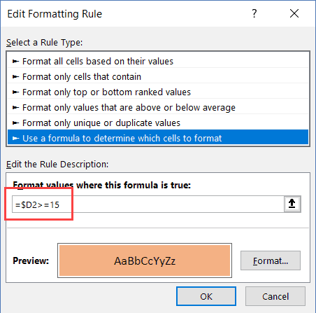
7. Click the ‘Format’ button. In the dialog box that opens, set the color in which you want the row to get highlighted.
8. Click OK.

This will highlight all the rows where the quantity is more than or equal to 15.

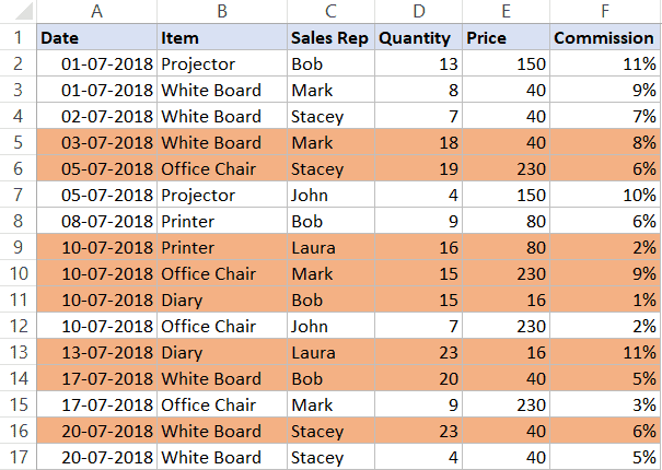
Similarly, we can also use this to have criteria for the date as well.

For example, if you want to highlight all the rows where the date is after 10 July 2018, you can use the below date formula:

=$A2>DATE(2018,7,10)

Highlight Rows Based on a Multiple Criteria (AND/OR)

You can also use multiple criteria to highlight rows using conditional formatting.

For example, if you want to highlight all the rows where the Sales Rep name is ‘Bob’ and the quantity is more than 10, you can do that using the following steps:

1. Select the entire dataset (A2:F17 in this example).
2. Click the Home tab.
3. In the Styles group, click on Conditional Formatting.
4. Click on ‘New Rules’.
5. In the ‘New Formatting Rule’ dialog box, click on ‘Use a formula to determine which cells to format’.
6. In the formula field, enter the following formula: =AND($C2=”Bob”,$D2>10)
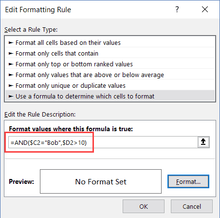
7. Click the ‘Format’ button. In the dialog box that opens, set the color in which you want the row to get highlighted.
8. Click OK.

In this example, only those rows get highlighted where both the conditions are met (this is done using the AND formula).

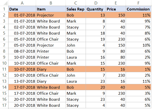
Similarly, you can also use the OR condition. For example, if you want to highlight rows where either the sales rep is Bob or the quantity is more than 15, you can use the below formula:

=OR($C2="Bob",$D2>15)

Click here to download the Example file and follow along.

Highlight Rows in Different Color Based on Multiple Conditions

Sometimes, you may want to highlight rows in a color based on the condition.

For example, you may want to highlight all the rows where the quantity is more than 20 in green and where the quantity is more than 15 (but less than 20) in orange.

To do this, you need to create two conditional formatting rules and set the priority.

Here are the steps to do this:

1. Select the entire dataset (A2:F17 in this example).
2. Click the Home tab.
3. In the Styles group, click on Conditional Formatting.
4. Click on ‘New Rules’.
5. In the ‘New Formatting Rule’ dialog box, click on ‘Use a formula to determine which cells to format’.
6. In the formula field, enter the following formula: =$D2>15
7. Click the ‘Format’ button. In the dialog box that opens, set the color to Orange.
8. Click OK.
9. In the ‘Conditional Formatting Rules Manager’ dialog box, click on ‘New Rule’.
10. In the ‘New Formatting Rule’ dialog box, click on ‘Use a formula to determine which cells to format’.
11. In the formula field, enter the following formula: =$D2>20
12. Click the ‘Format’ button. In the dialog box that opens, set the color to Green.
13. Click OK.
14. Click Apply (or OK).

The above steps would make all the rows with quantity more than 20 in green and those with more than 15 (but less than equal to 20 in orange).

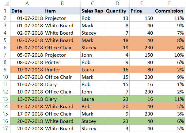
Understanding the Order of Rules:

When using multiple conditions, it important to make sure the order of the conditions is correct.

In the above example, the Green color condition is above the Orange color condition.

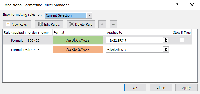
If it’s the other way round, all the rows would be colored in orange only.

Why?

Because a row where quantity is more than 20 (say 23) satisfies both our conditions (=$D2>15 and =$D2>20). And since Orange condition is at the top, it gets preference.

You can change the order of the conditions by using the Move Up/Down buttons.

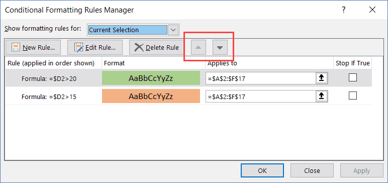
Click here to download the Example file and follow along.

Highlight Rows Where Any Cell is Blank

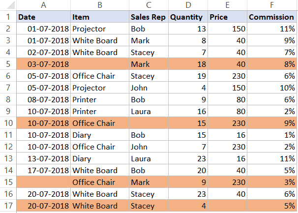
If you want to highlight all rows where any of the cells in it is blank, you need to check for each cell using conditional formatting.

Here are the steps to do this:

1. Select the entire dataset (A2:F17 in this example).
2. Click the Home tab.
3. In the Styles group, click on Conditional Formatting.
4. Click on ‘New Rules’.
5. In the ‘New Formatting Rule’ dialog box, click on ‘Use a formula to determine which cells to format’.
6. In the formula field, enter the following formula: =COUNTIF($A2:$F2,””)>0
7. Click the ‘Format’ button. In the dialog box that opens, set the color to Orange.
8. Click OK.

The above formula counts the number of blank cells. If the result is more than 0, it means there are blank cells in that row.

If any of the cells are empty, it highlights the entire row.

Related: Read this tutorial if you only want to highlight the blank cells.

Highlight Rows Based on Drop Down Selection

In the examples covered so far, all the conditions were specified with the conditional formatting dialog box.

In this part of the tutorial, I will show you how to make it dynamic (so that you can enter the condition within a cell in Excel and it will automatically highlight the rows based on it).

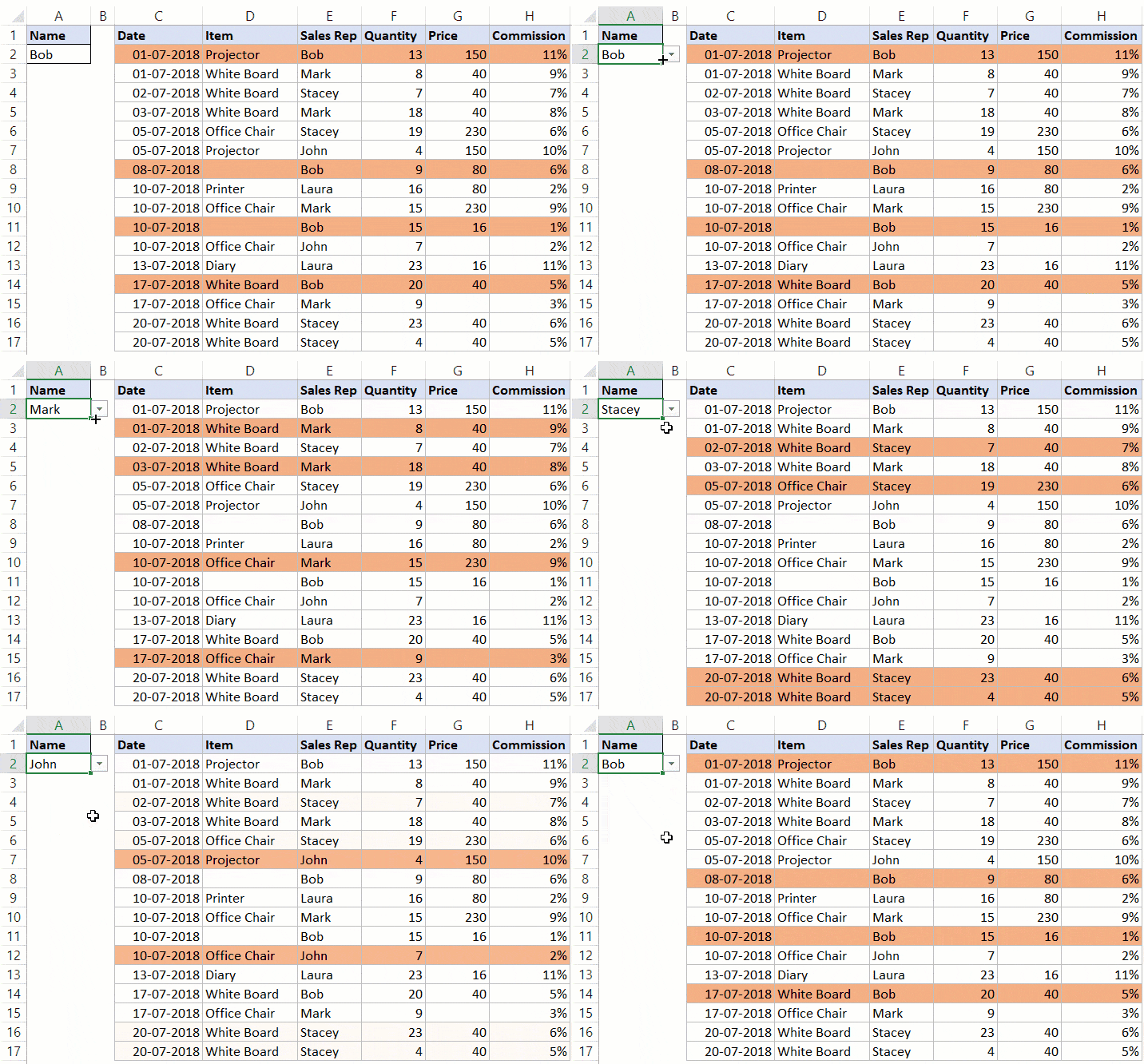
Below is an example, where I select a name from the drop-down, and all the rows with that name get highlighted:

Here are the steps to create this:

1. Create a drop-down list in cell A2. Here I have used the names of the sales rep to create the drop down list. Here is a detailed guide on how to create a drop-down list in Excel.
2. Select the entire dataset (C2:H17 in this example).
3. Click the Home tab.
4. In the Styles group, click on Conditional Formatting.
5. Click on ‘New Rules’.
6. In the ‘New Formatting Rule’ dialog box, click on ‘Use a formula to determine which cells to format’.
7. In the formula field, enter the following formula: =$E2=$A$2
8. Click the ‘Format’ button. In the dialog box that opens, set the color to Orange.
9. Click OK.

Now when you select any name from the drop-down, it will automatically highlight the rows where the name is the same that you have selected from the drop-down.

#evba #etipfree #kingexcel
📤You download App EVBA.info installed directly on the latest phone here : https://www.evba.info/p/app-evbainfo-setting-for-your-phone.html?m=1