Excel chart of Top / Bottom “N” values using RANK() function and Form controls

Ever fancied that you have large set of data and from it you can have a chart of top or bottom N values and better yet you have the ability to switch between chart of top N and bottom N values as easy as flicking the switch on/off?

Well this is what we are about to do today. This is one MUST know thing for those who want to make Excel dashboards as decision makers love to know the best and worst performing elements in specific KPI. Following is what we will get by the end of this tutorial:

View Contents [hide]

• Excel RANK() function – Intro
• Setting up the Data
• Setting up form controls
• Automating the process – RANK function revisited
• Setting up the chart
• Liked this charting tutorial? Check out these tutorials too:

Excel RANK() function – Intro

Sooner or later if you are into Excel dashboards this function will be your back pocket accessory. Lets understand what this function does:

RANK(number,ref,[order])

number: the number which you want to compare with others in the list or array to get ranked

ref: in simple words address to collection of numbers in a data set. This will definitely be a range.

order: an optional argument. This ranks the number in ascending or descending manner with respect to list. It can be zero 0 or one 1. By default it is 0.

Download Excel Tutorial Workbook

Click here to download the Excel file that serves the basic data needed to follow the steps in this tutorial

Setting up the Data

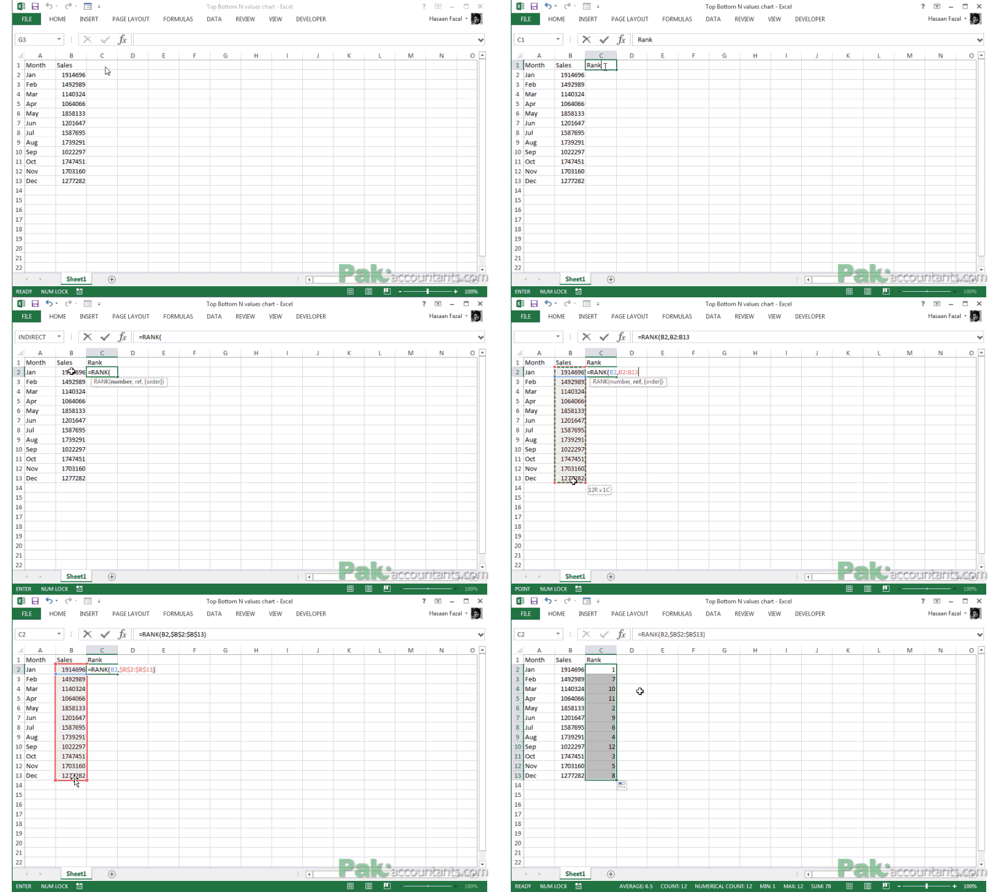
Step 1: Get the required data. In my case it is simple sales data of 12 months from January till December.

Step 2: In column C give a heading Rank or any other appropriate heading for understanding purposes. I gave Rank.

Step 3: As I have data starting in row 2 and also my rank column is also starting from same row, things are easy for me. Put the following formula in cell C2

=RANK(B2,$B$2:$B$13)

This formula is checking the value in cell B2 against other numbers in range B2 to B13 and according ranking them.

Double click the fill handle and it will populate the cells with ranks for each number in the sales column. As we have not mentioned the order argument, Excel will take it as Zero giving the lowest number to the highest value. In our case highest value is 1914696 therefore rank of 1 is given to this number.

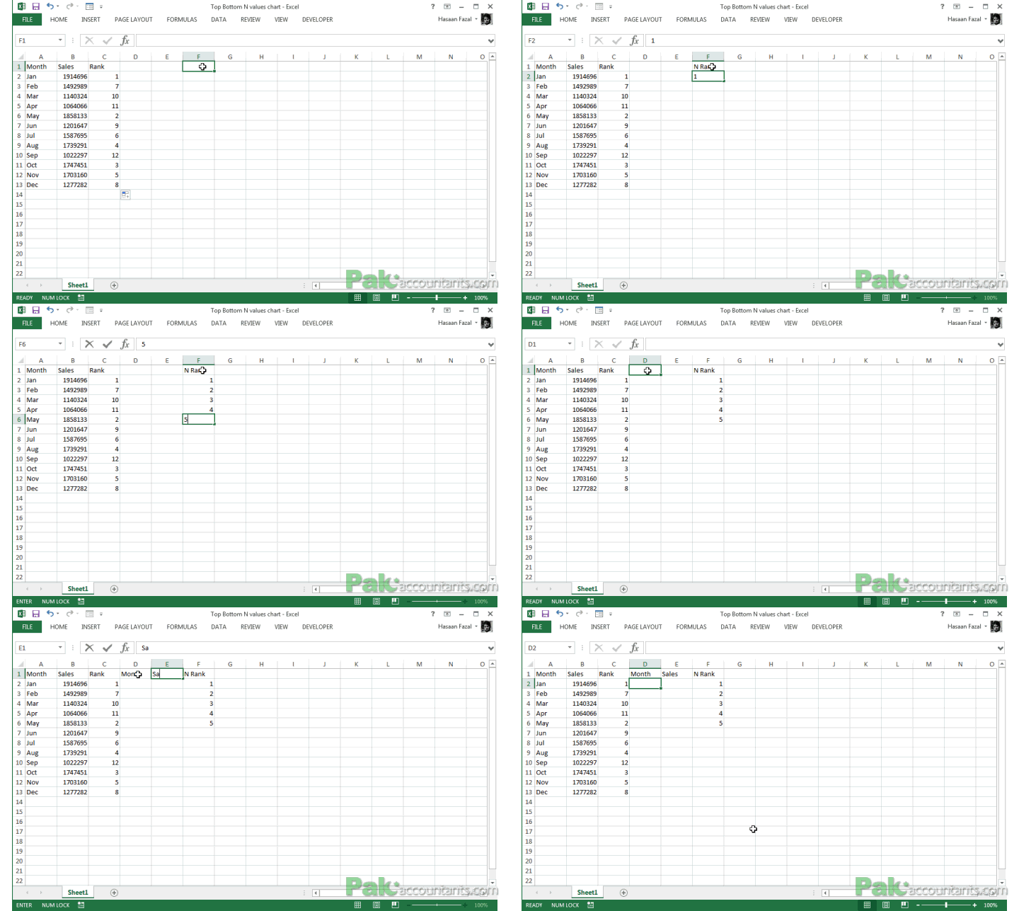
Step 4: Go to cell F1 and make a heading N Rank.

Step 5: Put 1 in cell F2, 2 in F3, 3 in F4, 4 in F5 and 5 in F6. 5 because we need top 5 or Bottom 5 from the sales data. If we want less or more we can adjust it here.

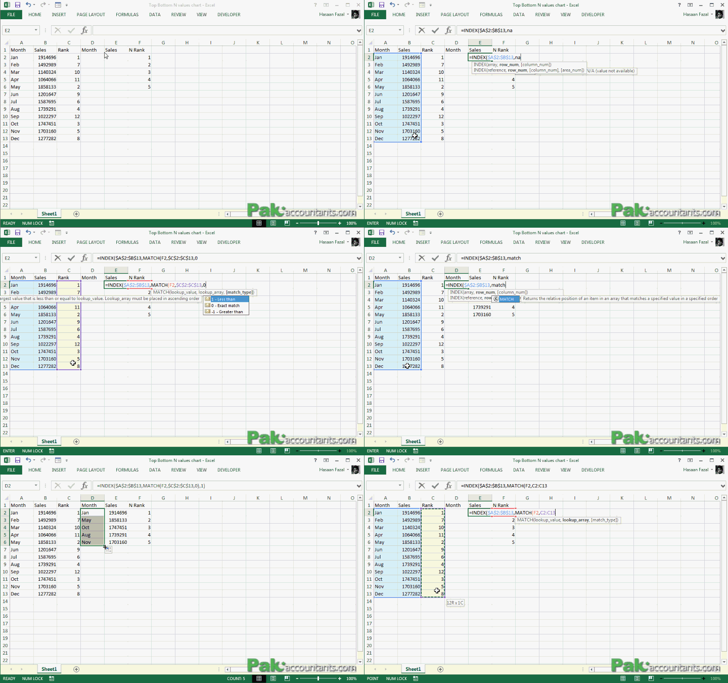
Step 6: Now we need sales value and corresponding month for each of the rank from 1 through 5. To get this we can use combo of INDEX and MATCH functions. Go to cell E2 and put this formula:

=INDEX($A$2:$B$13,MATCH(F2,$C$2:$C$13,0),2)

INDEX function fetches a certain value from the collection of data set. But we have to provide it with the row number and column number if we have more than 1 column in the data set. At the moment we are looking for sales value and we have selected the data in the range A2 till B13 and sales values are in second column. That is why we put in the value 2 which you can see in the end of the formula.

However, we still need the row number. For that we are using MATCH function. Remember column F has rank values. We want Excel to find the value in cell F2 in the range C2 through C13 and return the row number where it exists. Match function will serve with the row number.

Once we have this row number, INDEX number can now use it to fetch sales value as the only missing argument was row number to get the sales value. Don’t worry if INDEX + MATCH working is still alien to you. I will write about them sooner now.

Drag the fill handle down to populate the cells until cell E6.

Step 7: Now as we have sales value, we need corresponding months as well. To get that, go to cell D2 and put this formula:

=INDEX($A$2:$B$13,MATCH(F2,$C$2:$C$13,0),1)

It is the exact same formula as discussed above. The only difference is it has 1 at the end. As we are looking for months and months are listed in first column of range selected therefore, 1.

The following animation walk you through the above steps:

Now that we have the data set up to be used. Two things are still left:

1. Form controls
2. Chart

Setting up form controls

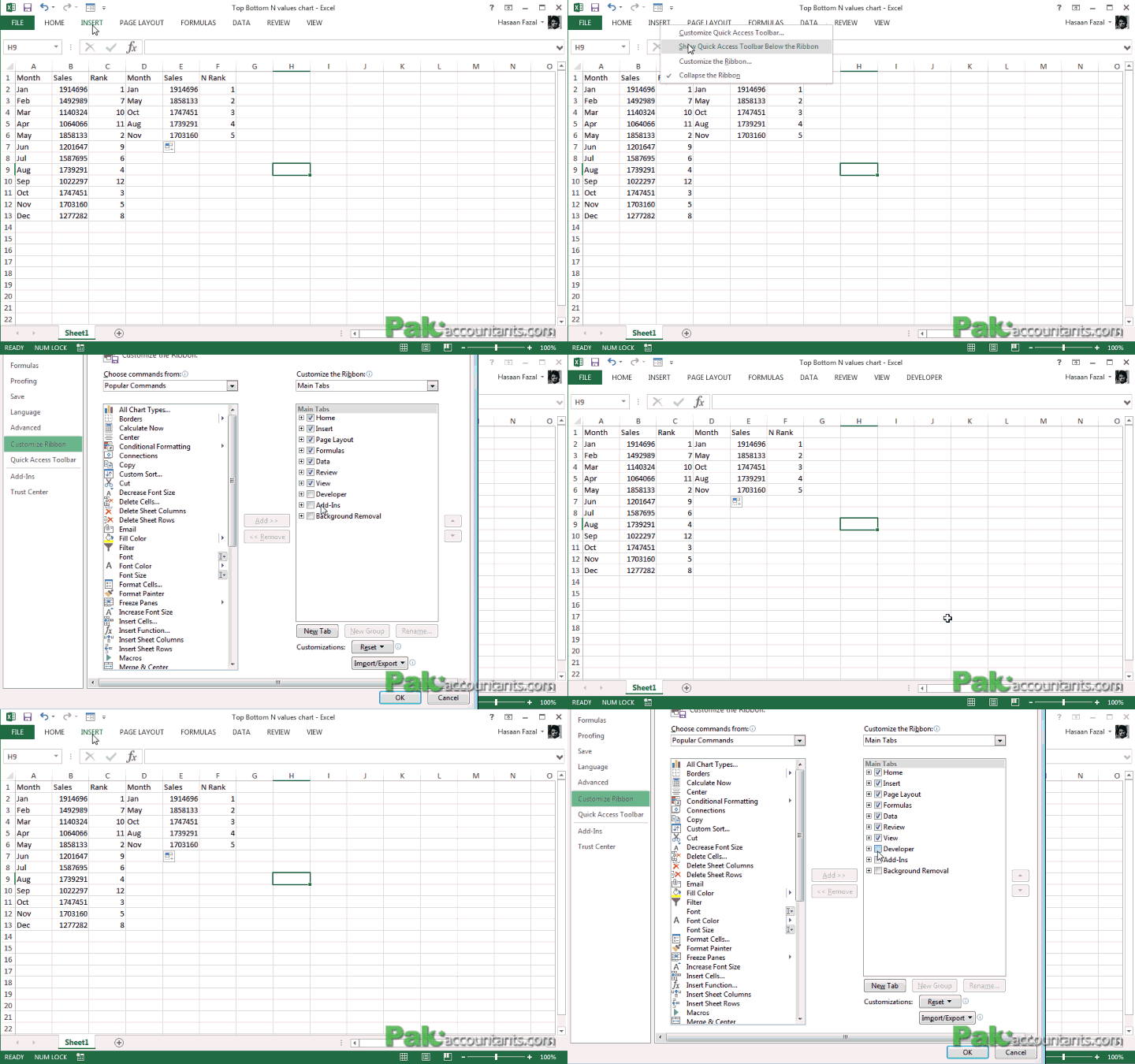
Step 1: Enable developer tab if its not already enabled. Have a look at the following animated walk through

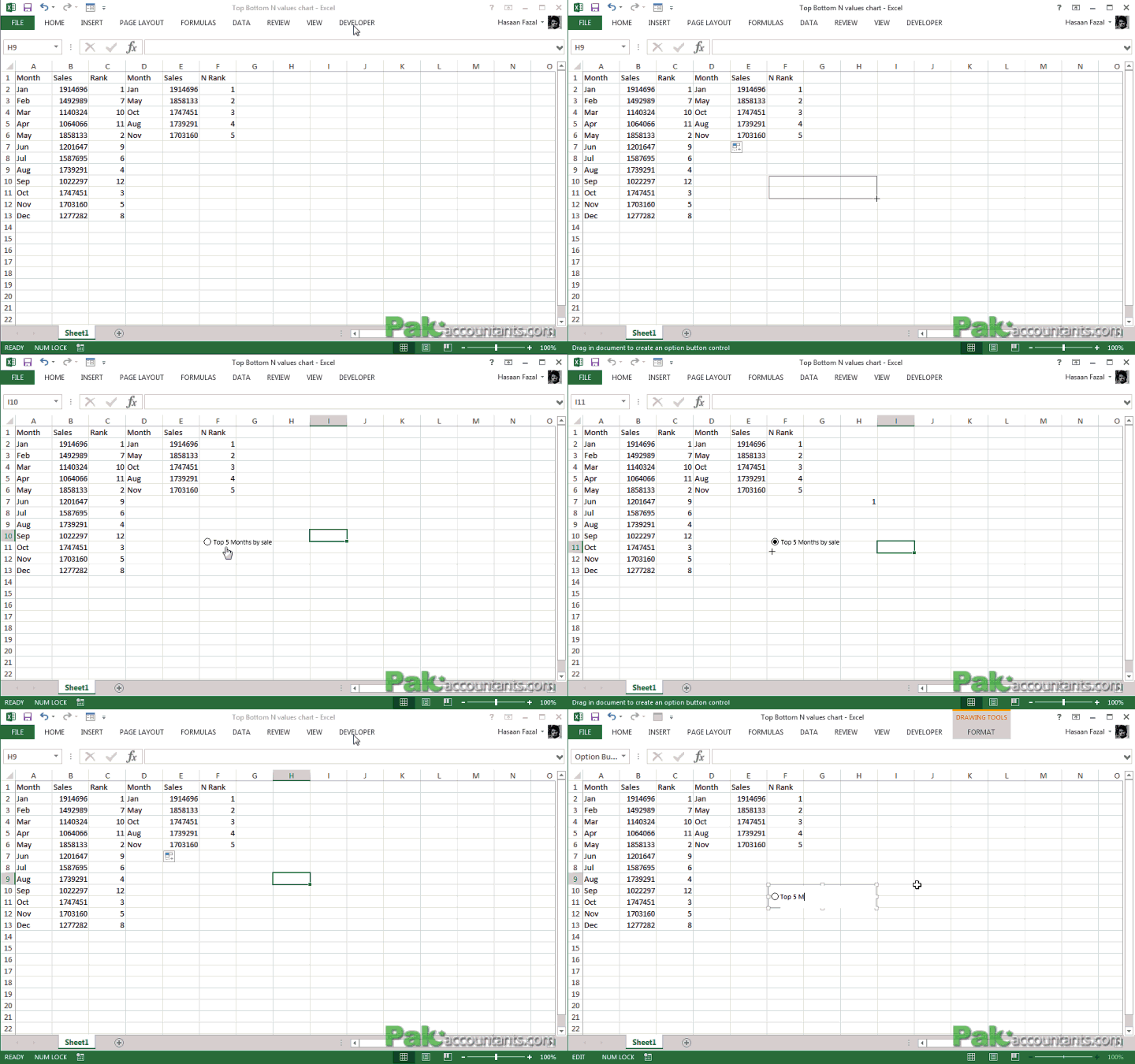
Step 2: Go to developer tab > controls group > click insert drop down button > under form controls > click option button. Draw the button. Don’t worry if its not perfect in first attempt you can adjust it later.

Step 3: Right click on inserted button > edit text and type Top 5 months by sale

Step 4: Right click again > format controls > in cell link put the absolute address to cell H7 i.e. $H$7. Click OK. Now that button is linked with cell H7.

Step 5: Insert another button following the step 2. And later change its text to Bottom 5 months by sale

Step 6: My second button was already linked to cell H7 but if your’s is not then you can do so by following step 4 above.

Now if you click either of the two buttons the value in cell H7 will change between 1 and 2. We can put this functionality to great use.

Following animation will walk you through swiftly through simple steps mentioned above:

Automating the process – RANK function revisited

As of now we have the list. The top 5 months by sales. However, we are still missing the bottom 5 months by sales. We can easily get it by changing one argument in function mentioned in Rank column. Remember the order argument in the RANK function? Its time to use it!

We can get the top 5 and bottom 5 values with the order argument and now it will make much more sense why we used INDEX and MATCH function.

Go to cell C2 and change the existing formula to this:

=RANK(B2,$B$2:$B$13,IF($H$7=1,0,1))

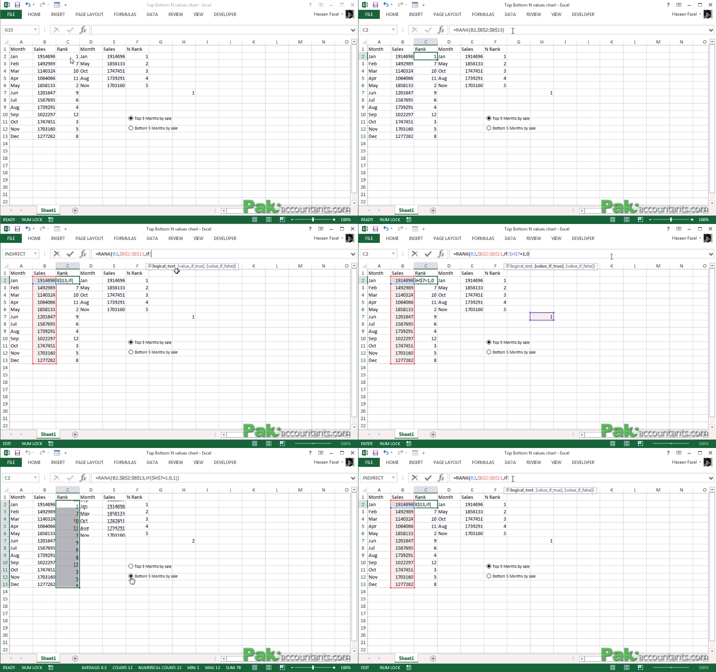
Notice the difference between this formula and the old one? Let me put the two formula together for better understanding:

Old formula: =RANK(B2,$B$2:$B$13)

New formula: =RANK(B2,$B$2:$B$13,IF($H$7=1,0,1))

We have added this part: IF($H$7=1,0,1)

Remember we have values changing 1-2 in cell H7 if we click the buttons we inserted? We are going to use this to automate our order argument. So if H7 has 1 in it the IF function will send out 0 to the formula and if not than 1. This way we will have the order change from ascending to descending and thus ranking the top 5 and bottom 5.

Drag the fill handle to populate the whole range with updated formula. Now click the buttons and see the ranking changing its order in the column instantly. And that will also change the values in our second list containing Top / Bottom N values.

Now the chart plotted using such dynamic data will change too. Aaahhh I LOVE details! 

Setting up the chart

Select the data in the list (the second data set containing 5 entries) and go to Insert tab > charts group > line charts > 2D column charts > clustered column charts and it will insert the chart. Now arrange it as you desire and click the buttons and see the graph dance to your clicks!

Awesome!

So here you have working breathing changing Top 5 and Bottom 5 months of sales plotted on a graph ready to be switched at your click’s notice. With a small cosmetic uplift this is what I have:

#evba #etipfree #kingexcel
📤You download App EVBA.info installed directly on the latest phone here : https://www.evba.info/p/app-evbainfo-setting-for-your-phone.html?m=1