Dynamic Dependent Dropdown by Data Validation

Dynamic Dependent Dropdown by Data Validation

by MF

So many D. 

This is a continuation of the previous post:

Not all teachers are eligible to all classes.  e.g. only Iris and David are eligible to deliver Class F, would it be feasible to have only Iris and David on the dropdown list, in the ascending order of hours assigned?

Yes it is.

You may download a Sample File  to follow along.

It requires three helper tables.  Let’s set them up one by one.

 1) Set up the Eligibility Table (Table 1) to show which teacher is eligible to which class(es).  This is quite straight-forward.

 2) Riding on the Dynamic list we set up before (see previous post for details), set up Table 2 to determine the “Show up sequence” of eligible teacher(s) for each class.  

Formula used:

L3 =IF(INDEX(L$13:L$18,MATCH($K3,$K$13:$K$18,0))*$J3=0,””,

INDEX(L$13:L$18,MATCH($K3,$K$13:$K$18,0))*$J3) ‘Copy down and across

The latter part of the formula INDEX(L$13:L$18,MATCH($K3,$K$13:$K$18,0))*$J3

is used to determine if a teacher is eligible for a class; and then assigned a number from smallest to largest to that teacher according to the “Show up sequence”, i.e. number of hours assigned.

The IF function is used to eliminate the result of “0” which means the teacher is not eligible for the class.

 3) To set up the final dynamic list (Table 3) according to the result from Table 2

Formula used:

• L23 =IFERROR(INDEX($K$3:$K$8,SMALL(L$3:L$8,$K23)),””)  ‘Copy down and across

This formula establishes lists of eligible teacher with corresponding show up sequence according to the hours assigned.  IFERROR is used to replace possible error with “”, thus “#NUM!” won’t appear on the list.

Overview of the three Tables

Set up the Data Validation: 

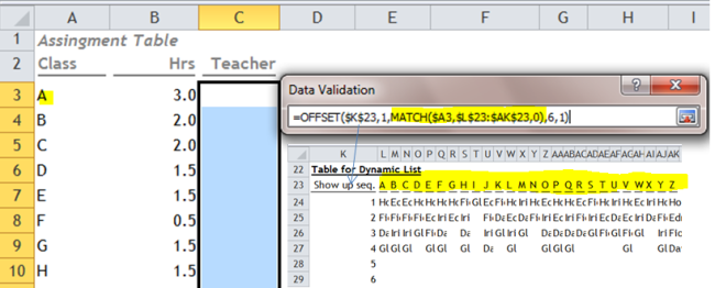
Use the dynamic results from Table 3 by using OFFSET as source for Data Validation.

1. Select Range C3:C28
2. On Ribbon, Data Tab –> Data Validation
3. Allow “List”
4. Source: =OFFSET($K$23,1,MATCH($A3,$L$22:$AK$22,0),6,1)

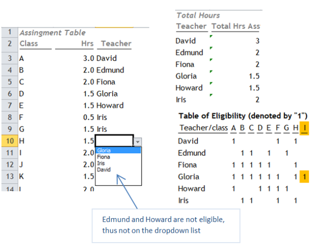
Let’s test the drop down.

It is working!   Try one more.

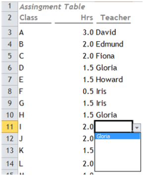
See, only Gloria is on the list as she is the only eligible teacher for class I.

Final step is to hide columns J:AK to have a clean look of the spreadsheet.

What the OFFSET formula does?

The syntax is as follow:

=OFFSET(reference,rows,cols,height,width)

Take our formula as an example:

=OFFSET($k$23,1,1,6,1)

Meaning: Starting from $k$23, move down 1 row, then move 1 column to the right, select a range of 6 rows height and 1 column width.  As a result, it refers to the range L24:L29 {“Howard”;”Flora”;”David”;”Gloria”;””;””}.  And this is the dynamic list for Class A.

Note: the cols argument is controlled by the Match function, which make the result dynamic.  The Match portion returns the relative position in Table 3 for the corresponding class.  E.g. In cell A3, the class is A.  The Match functions then return 1 as a result.  If the class is B, then it returns 2 as a result, etc.

So for Class A, the OFFSET formula refers to the Range L24:L29; for class B, the formula refers to the range M24:M29 and so on and so forth.

Well, a bit complex?!  Maybe.  Nonetheless, I am more intended to show you the possibility of using various Excel Functions collaboratively for something nice.  Let’s keep exploring.

Debra Dalgleish just shared another great article <Dependent Drop Down Lists With Tables>, where you can learn another technique in preparing depending drop down list through data validation and Tables.

#evba #etipfree #kingexcel
📤You download App EVBA.info installed directly on the latest phone here : https://www.evba.info/p/app-evbainfo-setting-for-your-phone.html?m=1