Do 60 What-If Analyses with a Sensitivity Analysis

January 01, 2020 Mr King Excel Tips,

Do 60 What-If Analyses with a Sensitivity Analysis

Goal Seek lets you find the set of inputs that lead to a particular result. Sometimes, you want to see many different results from various combinations of inputs. Provided that you have only two input cells to change, the Data Table feature will do a sensitivity analysis.

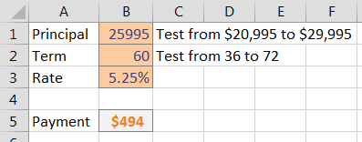
Using the loan payment example, say that you want to calculate the price for a variety of principal balances and for a variety of terms.

You have a three-variable model for car payment. You want to do a sensitivity analysis with Principal from $21K to $30K and Term from 36 to 72 months.

Make sure that the formula you want to model is in the top-left corner of a range. Put various values for one variable down the left column and various values for another variable across the top.

The formula calculating payment has to be the top-left corner of the sensitivity analysis. Below that, enter 21000 to 30000 in 1000 unit increments. To the right of the top left cell, enter 36, 48, 54, 60, 66, 72.

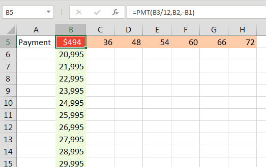
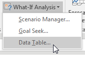
From the Data tab, select What-If Analysis, Data Table....

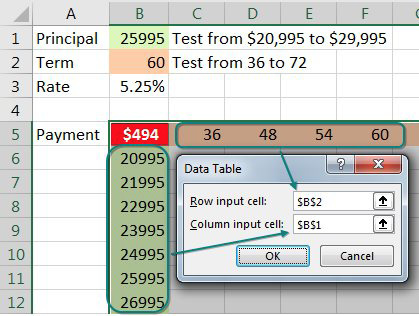
On the Data tab, under What-If Analysis, choose Data Table.

You have values along the top row of the input table. You want Excel to plug those values into a certain input cell. Specify that input cell for Row Input Cell.

You have values along the left column. You want those plugged into another input cell. Specify that cell for the Column Input Cell.

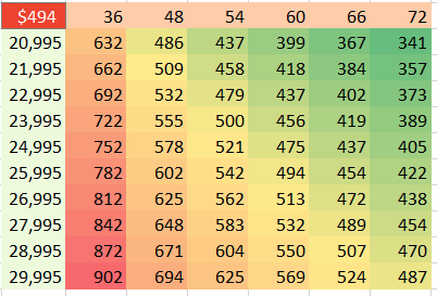
The data table dialog asks for a Row Input Cell and a Column Input cell. Since you have monthly terms across the top row, those should get plugged in to B2. The loan principal along the left column should be plugged in to B1.

When you click OK, Excel repeats the formula in the top-left column for all combinations of the top row and left column. In the image below, you see 60 different loan payments, based on various inputs.

The results of the sensitivity analysis range from a low of $341 a month to $902 a month. In this screen shot, a color scale marks the highest numbers in red.

Note

I formatted the table results to have no decimals and used Home, Conditional Formatting, Color Scale to add the red/yellow/green shading.

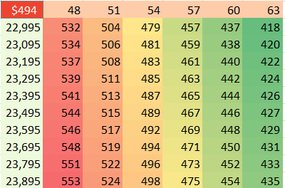
Here is the great part: This table is “live.” If you change the input cells along the left column or top row, the values in the table recalculate. Below, the values along the left are focused on the $23K to $24K range.

Change the numbers in the top row and left column and the data recalculates. In this image, with months from 48 to 63 and prices from 23K to 24K, the monthly car payments range from $418 to $553.

Tip

You can build far more complex models and still use a data table. In my podcast 2141 "Will Asteroid Bennu Strike the Earth" on YouTube, I had a model with 100K NORM.INV and 100K VLOOKUP. Those 200,000 formulas were sent to a SUM function that summarized them. I used a Data Table to run those 200,001 formulas 100 times. The whole thing recalcs in about 11 seconds.

#evba #etipfree #kingexcel
📤You download App EVBA.info installed directly on the latest phone here : https://www.evba.info/p/app-evbainfo-setting-for-your-phone.html?m=1