Count paired items in listed combinations

Generic formula 

=COUNTIFS(range,"*"&$item1&"*",range,"*"&item2&"*")

Explanation 

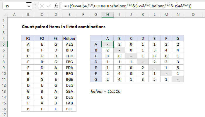
To build a summary table with a count of paired items that appear in a list of existing combinations, you can use a helper column and a formula based on the COUNTIFS function. In the example shown the formula in cell H5 is:

=IF($G5=H$4,"-",COUNTIFS(helper,"*"&$G5&"*",helper,"*"&H$4&"*"))

where "helper" is the named range E5:E24.

Note: this formula assumes items don't repeat in a given combination (i.e. AAB, EFE are not valid combinations).

How this formula works

We want to count how often items in columns B, C, and D appear together. For example, how often A appears with C, B appears with F, G appears with D, and so on. This would seem like a perfect use of COUNTIFS, but if we try to add criteria looking for 2 items across 3 columns, it isn't going to work.

A simple workaround is to join all items together in a single cell, then use COUNTIFS with a wildcard to count items. We do that with a helper column (E) that joins items in columns B, C, and D using the CONCAT function like this:

=CONCAT(B5:D5)

In older versions of Excel, you can use a formula like this:

=B5&C5&D5

Because repeated items are not allowed in a combination, the first part of the formula excludes matching items. If the two items are the same, the formula returns a hyphen or dash as text:

=IF($G5=H$4,"-"

If items are different, a COUNTIFS function is run:

COUNTIFS(helper,"*"&$G5&"*",helper,"*"&H$4&"*")

COUNTIFS is configured to count "pairs" of items. Only when the item in column G and the corresponding item from row 4 appear together in a cell is the pair counted. A wildcard (*) is concatenated to both sides of the item to ensure a match will be counted no matter where it appears in the cell.

#evba #etipfree #kingexcel
📤You download App EVBA.info installed directly on the latest phone here : https://www.evba.info/p/app-evbainfo-setting-for-your-phone.html?m=1