Complex Validation Using a Formula

January 07, 2020 Mr King Excel Tips,

Complex Validation Using a Formula

The method previously explained in Excel 2019: Dependent Validation using Dynamic Arrays is fine if you have Dynamic Arrays. But a lot of people running perpetual versions of Excel won't have Dynamic Arrays for years. Other published methods for Dependent Validation require a new named range for every possible choice in the first and second drop-down.

I was doing a seminar in Mobile, Alabama and several people there wanted to set up a three-level validation, but they did not care about having drop-downs to choose from. "I just want to validate that people are typing the correct values."

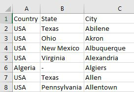
Rather than use the option to allow a list, you can set up custom validation using a formula. Say that you have a table with hundreds of valid selections.

A validation database with Country, State, and City.

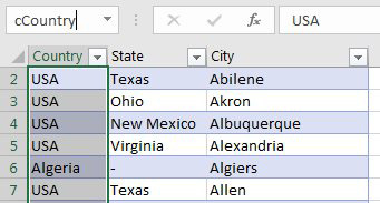
If you think that your list will grow over time, format it as a Table using Ctrl+T.

Set up a named range for each of the three columns. This step is necessary so you can refer to each column and the names will grow as the table grows.

Select A2:A551. In the Name Box, type cCountry and press enter.

Make the whole validation database into a table using Ctrl+T. But then, select the countries in A2:A999 and type a name in the name box of CCountry.

Name B2:B551 as cState. Name C2:C551 as cCity.

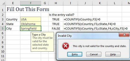
Here is the area where you want people to type a Country, State, and City.

It is always easier to build and test your formulas for conditional formatting and validation in a cell first. Take a look at the formulas shown below to test each of the entries.

Instructions in the worksheet say to Fill Out This Form. There are three cells where people type Country, State, and City. The formula to make sur Country in F3 is correct is: =COUNTIF(cCountry,F3)>0. The formula to validate State in F4 is: =COUNTIFS(cCountry,F3,cState,F4)>0. The formula to validate City is =COUNTIFS(cCountry,F3,cState,F4,cCity,F5)>0. Each of these will return TRUE if the entry is valid.

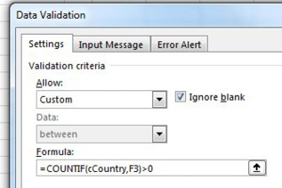
Once those formulas are working, edit cell H3. Using the mouse, select the characters in the formula bar and press Ctrl+C to copy. Select F3 and press Alt+D L to open the Data Validation drop-down. In the Allow box, choose Custom. This will reveal a Formula box. Paste your formula in that box.

In Data Validation, open the Allow box and choose Custom. Type a formula of =COUNTIF(cCountry,F3)>0

Optionally, fill out an Input Message and Error Alert. Repeat to put the H4 formula as the validation for F4 and the H5 formula for validation for F5. The result: it will prevent a wrong entry.

When you select the City cell, a tooltip appears with: Type a City. The City must be valid for the selected state and country. When you type something wrong in the cell, an Error Alert says Invalid City: The City Is Not Valid For the Country and State.

#evba #etipfree #kingexcel
📤You download App EVBA.info installed directly on the latest phone here : https://www.evba.info/p/app-evbainfo-setting-for-your-phone.html?m=1