Restructuring (Normalizing) data for Pivot tables using Pivot tables – How To

Last time I discussed the use of Power Query to restructure data for pivot table purposes if it is not arranged in columnar format. Today we will be learning how to normalize the data for pivot table purposes using pivot tables! Yes you read it right. We will use pivot tables to get the data straight to use it again for pivot tables. Don’t worry it is not like pivoting your head full circle.

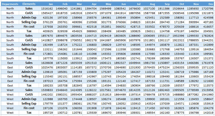
The data example that we will be restructuring is the same as we used to solve using power query technique. Here is the snapshot of what it looks like in its raw form:

So lets tame it!

Download Excel Tutorial workbook

For the purpose of this tutorial and to better understand the steps discussed later in this tutorial, download this Excel tutorial file and follow the steps.

Step 1: Right click on quick access toolbar > click customize quick access toolbar. A new window will open. From “Choose commands from” drop down select “All commands”. Scroll down and select Pivot table and Pivot chart wizard. Click Add button and it will add the command in QAT.

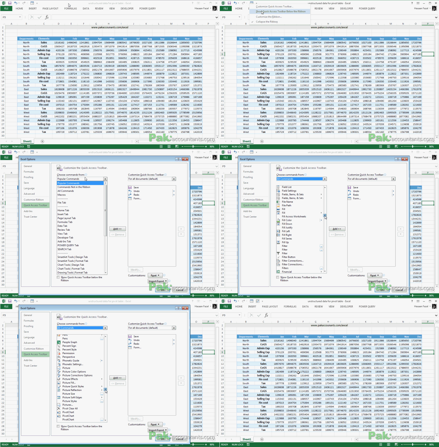
Step 2: Download and open the tutorial file. Right click on column D header and insert a new column. In cell D6 put the following formula:

=C6&”~”&B6

Double click the fill handle to populate the cells downward with the same formula. This formula has concatenated two cells in one and I have added “~” sign between them. You will understand the reason of it in a minute.

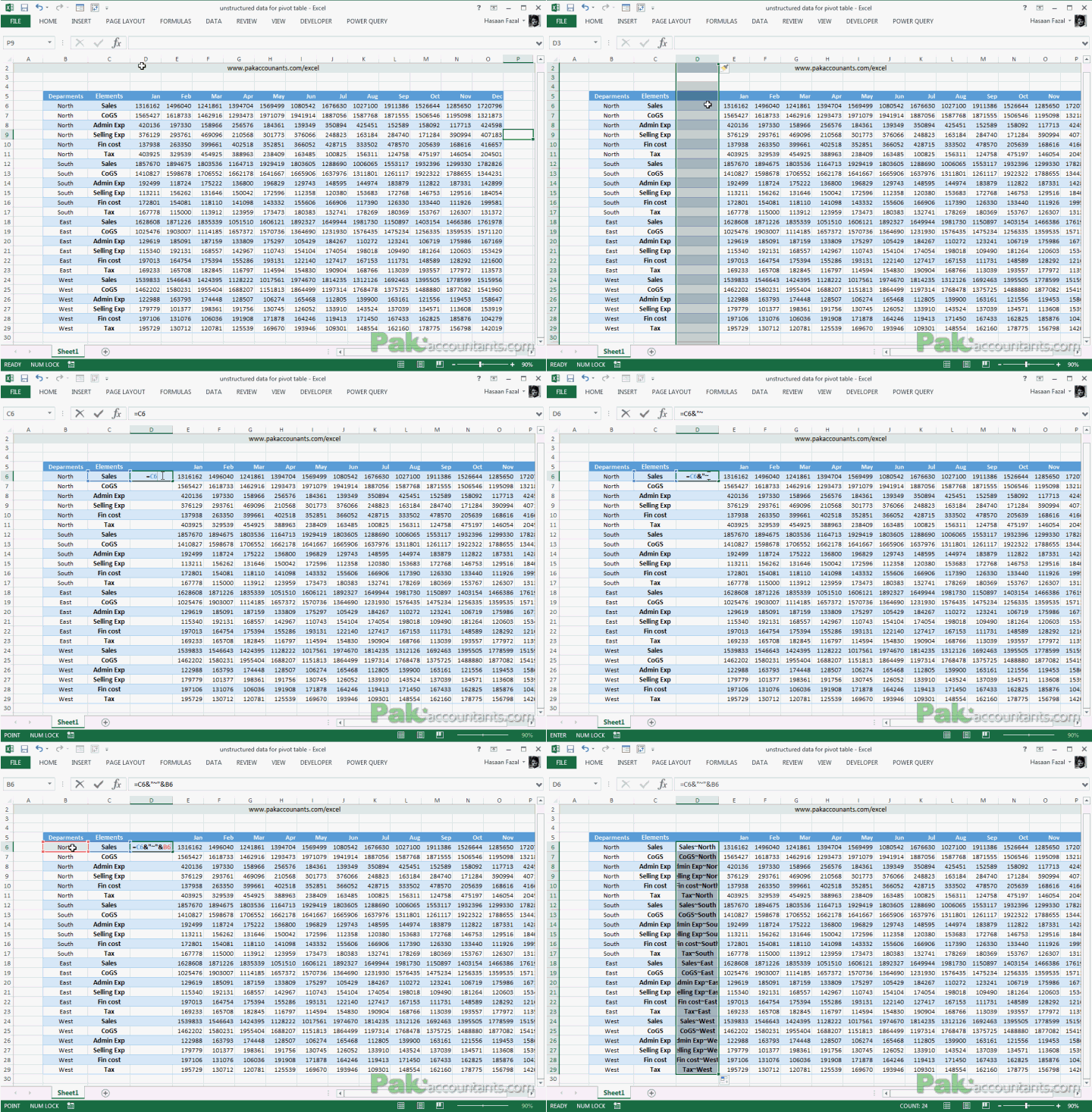
Step 3: Select the data range between column D and P leaving the first two column. Click the newly added button in the quick access toolbar

Step 4: A new dialogue box will open. Select “multiple consolidation ranges” option and click Next button

Step 5: Select “I will create the page fields” option. Select the same range again (from column D to P) and click “Add” button. Click Next button afterwards and then click Finish button.

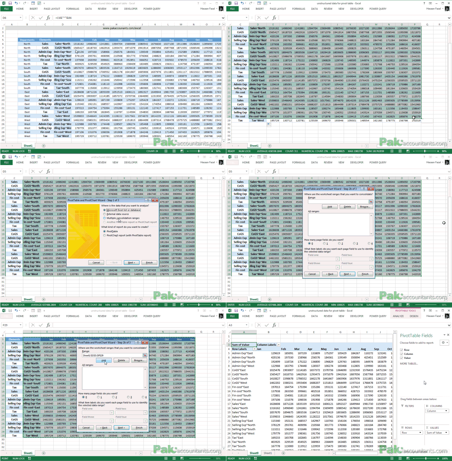
Step 6: A pivot report/table will be inserted in a new worksheet. Uncheck row/column options leaving only the value option selected under pivot table field options.

Step 7: Double click on the value figure to invoke drill down report.

Step 8: Select column A by left clicking the column header. Now press and hold right click on the edge of selection. While keep pressing down the right mouse button move the column to the right into column D and select “Shift right and move”. This will move the whole column to the farthest right.

Step 9: While column still selected go to Data tab > Data tools group > click text to column button.

Step 10: Select “Delimited” option and click Next button. Uncheck all options and check only “others” and in the input field type ~ sign and click Next button and then Finish button.

A new column will be added splitting the columns we joined at the very first place. Rename the new column “Departments”. Rename the “columns” named column with Months

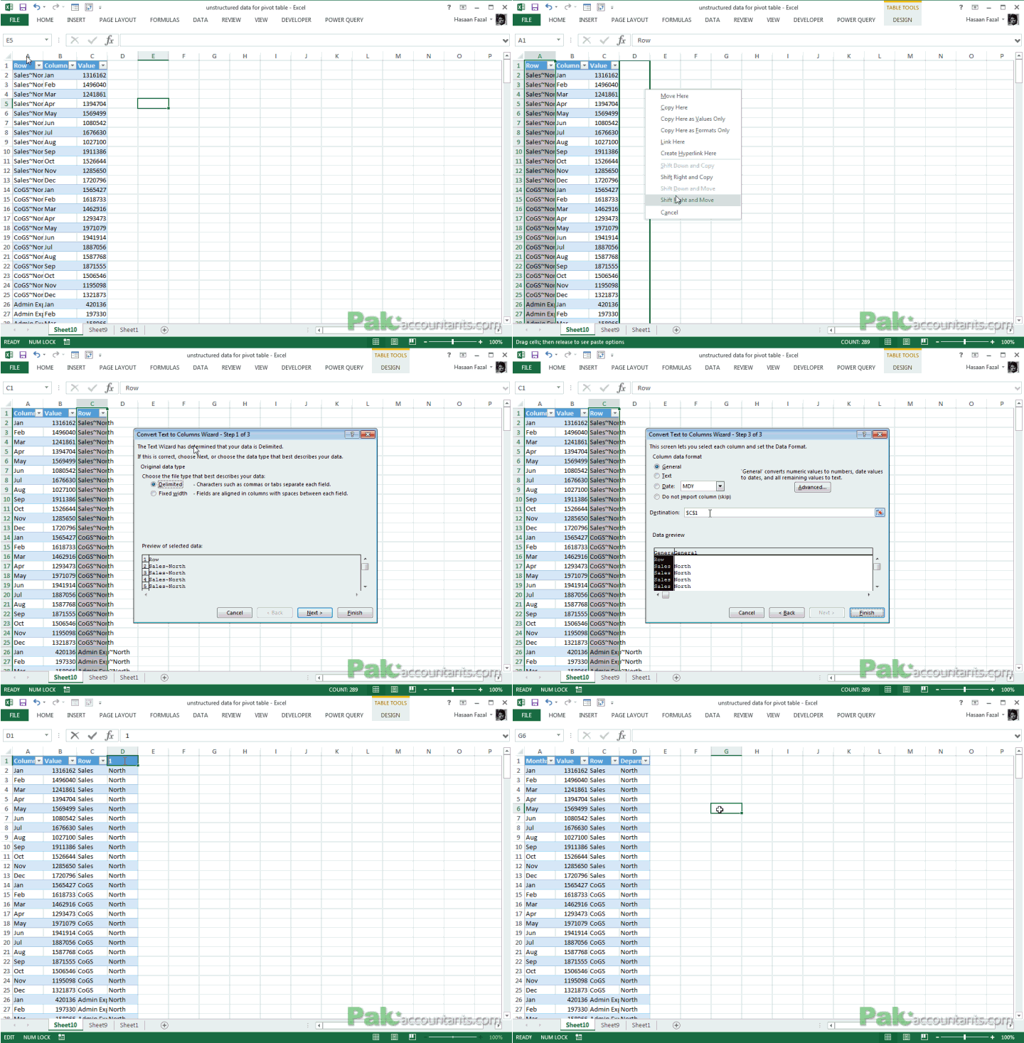
Our task is half complete. Yay!

Step 11: Have an active cell within the table and press Ctrl+A to select the table. Go to Insert tab > tables group > click pivot tables button and click OK. A new pivot table/report will be inserted in the new worksheet.

Step 12: Move:

1. Row field in the columns box
2. Months field in the rows box followed by Departments field in the rows box (below Months field)
3. Value field in the values box

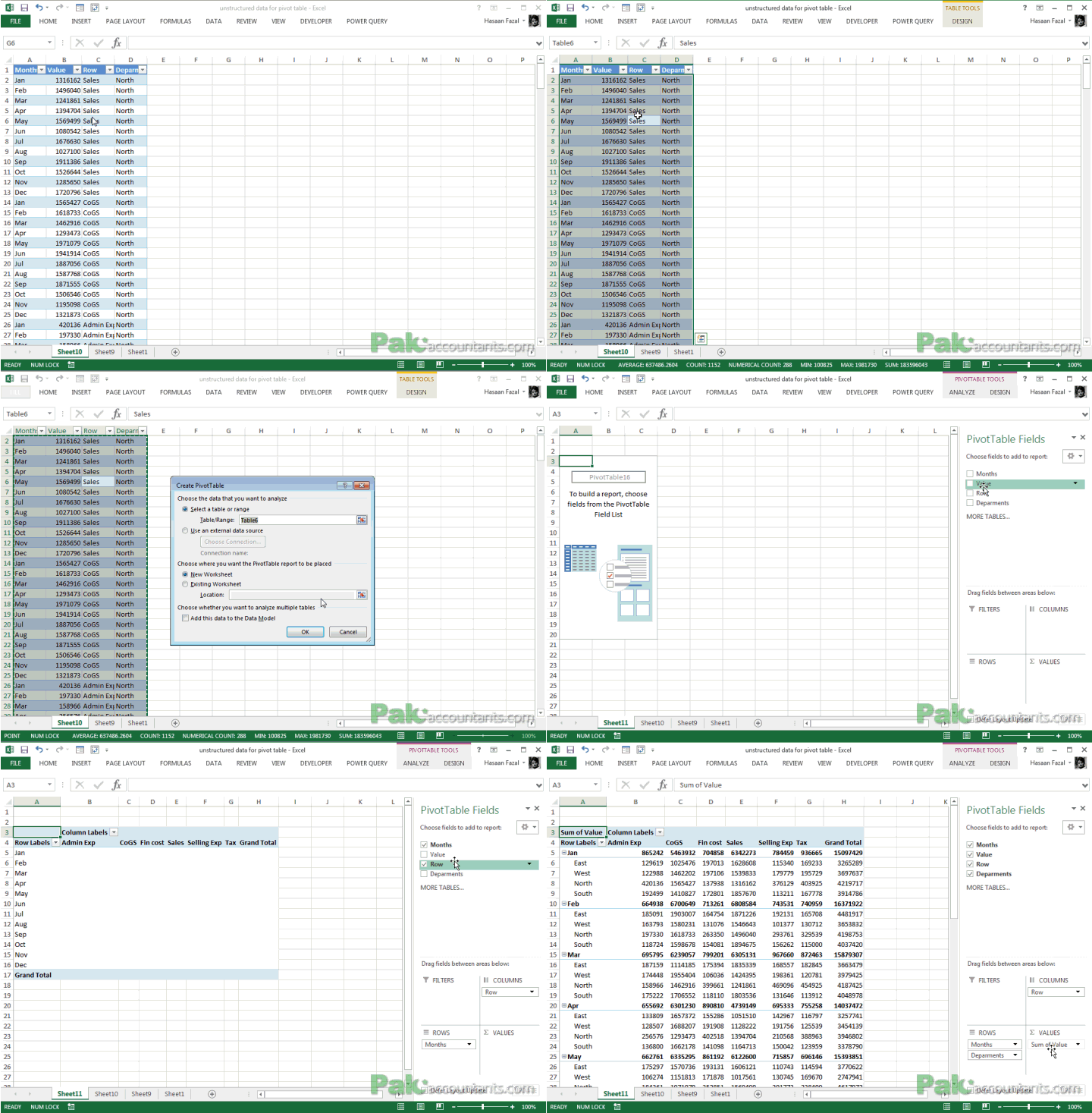
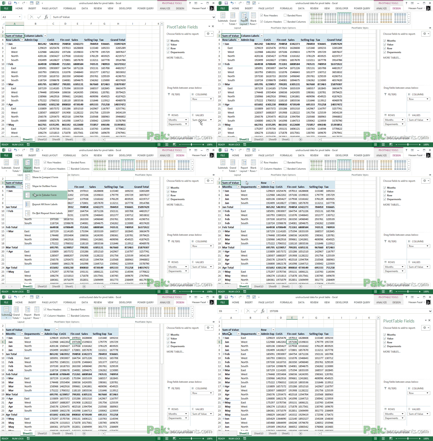
Step 13: Go to Design tab > layout group > click report layout drop down button > click show in tabular form.

Step 14: Again, go to Design tab > layout group > click report layout drop down button > click repeat all item labels

Step 15: Design tab > layout group > grand totals drop down button > off for rows and columns. In case subtotals are showing then turn the subtotals off as well.

Step 16: Select the table and copy the data. Insert a new worksheet and paste.

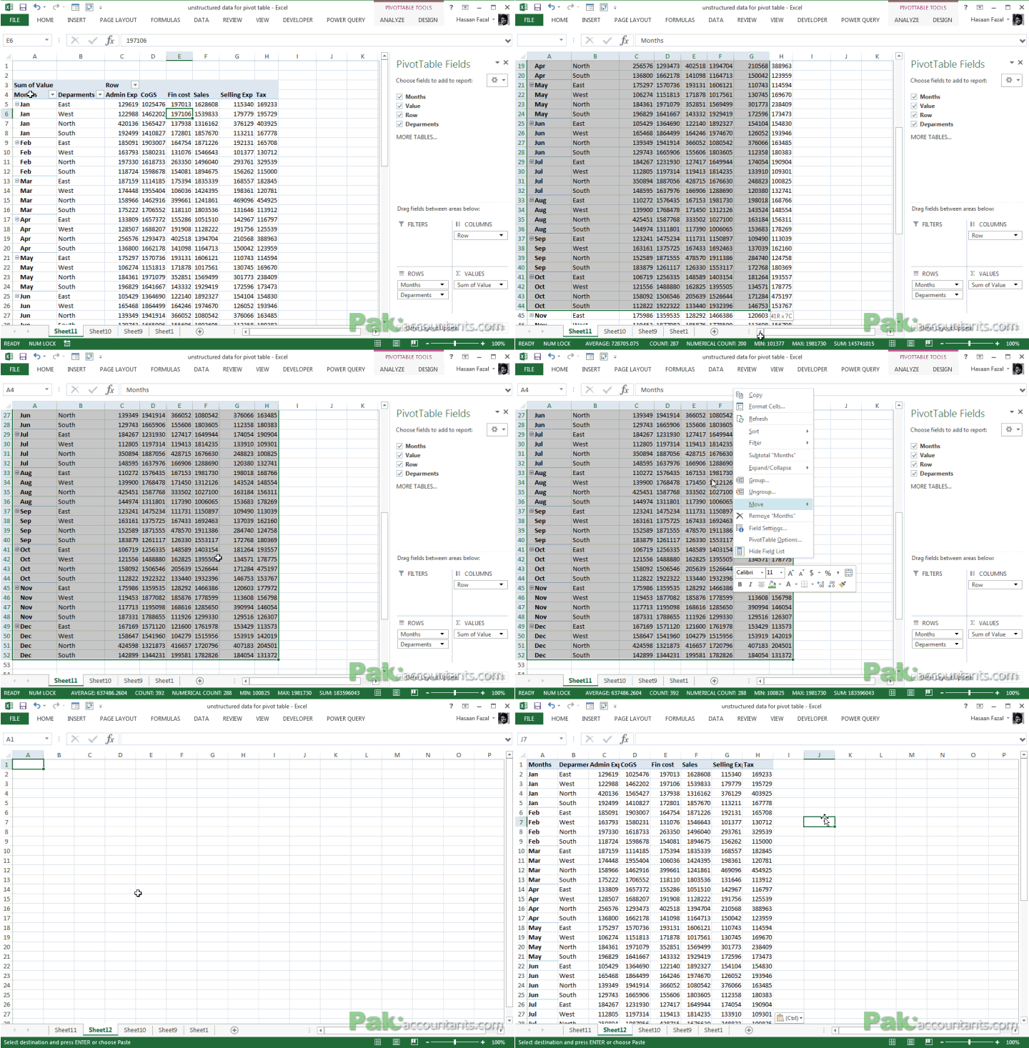
Done! You have the data all ready for pivot tables! Insane right? Its like using mangoes to cut mangoes!